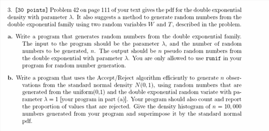
Project one. Problem Three. Mathematics 502 Probability and Statistics

Nasser Abbasi, September 26,2007. California State University, Fullerton

Problem 3 part (a)

We are asked to generate R.V's from . We note as shown in the problem itself, that R.V. X can be written as product of 2 R.V WT where Wis ±1 with probability each. Hence to generate R.V. we do the following. We generate n R.V. from uniform distribution [0,1] using Mathematica random number generator. Then we check if each number is or not, and we generate 1 or -1 as the case may be. We then generate n random variables from the exponential distribution, which we know how to do from part (a). Then we multiply the above 2 vectors, element wise, with each others. The first vector being the vector of 1's and -1's. And the second vector being the RV's from the exponential distribution.  This is the algorithm

Algorithm
Input: λ,n (number of random variables to generate)
output: list of random numbers which belong to density

Seed the random number generator with unique value for us.
A = Generate n random numbers from the exponential distribution with parameter λ (CALL problem 1 part(a) with the input λ,n) This uses method and uniform random number generator as well.
B = Generate n random numbers from uniform random number generator [0,1]

FOR i in 1..n LOOP  -- Note: This is algorithm view. In code 'vectored' operation is used.
        IF B(i)<.5 THEN
            B(i) = 1
         ELSE
            B(i) = -1
         END IF
END LOOP

result = B * A

Now generate a histogram from the result above.
The following function implements the above algorithm

Code Implementation

Define the function which was derived earlier. This is the inverse of the CDF of the exponential density function

In[208]:=

In[210]:=

In[211]:=

In[212]:=

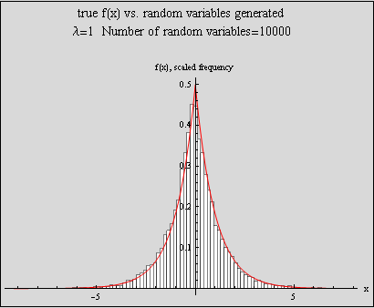
Test the above function by plotting the histogram generated for say n=10000 overlaid by the true double exponential density function.
First, define the double exponential function

In[213]:=

Now do the overlay plot

This function makes a histogram which is scaled to be used to overlay density plots, or other functions.
Input:  originalData: this is an array of numbers which represents the data to bin
          nBins: number of bins
output: the histogram itself but scaled such that area is ONE

In[214]:=

In[216]:=

Out[219]=

Problem 3 part(b)

In this part, we need to generate a list of r.v's that belong to normal distribution N(0,1), using uniform random number generator U[0,1] and using the random numbers generated from the double exponential density function in part (a) above. We are asked to use the accept/reject method.
First the method is explained, then the algorithm outlined, then the implementation shown and a test case given, then a GUI interface written to test the algorithm for different parameters values.

Accept/Reject algorithm
input: n (number of random variables to generate)
        λ (the exponential density parameter)
        f(x) the density function for random variable X which we wish to generate random variables
        (x) the density which we will use to help in generating the random variables from (x). This density is such that it is easy to generate random variables from. Much easier that from f(x) and that is why it was selected.
output: list of random numbers of length n from f(x)

Step 1: Find C. Where To solve this, this is the algorithm
           Algorithm for step 1:  Let (since double exponential is symmetric, I'll use one sided version). Let . Now find the ratio Now find where the maximum of this ratio is using normal calculus method:  Take the derivative w.r.t. x and set it to zero. Solve the resulting equation for x. Evaluate the ratio at this root. This gives C.   We find that C=1.31549   The following few lines of code finds C:

In[220]:=

Out[223]=

Step 2: Now that we found C in step 1, then the envelop function becomes
Step 3: seed the number random generator
            initialize an array d of size n to contain all the accepted random numbers generated
            initialize counter number_accepted=0
            WHILE number_accepted < n DO
                 generate  r.v. from U[0,1] call it u.  
                 Generate  r.v. from double exponential density (using part(a)) call this x
                 IF u*C* THEN
                     d[i]=x
                     number_accepted++
                 END IF
             END LOOP
   Step 4: Now array d contains the n random numbers generated from the normal density N[0,1].  Make histogram and overlay it over N[0,1]

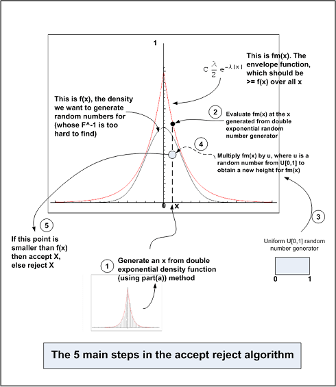
Diagram showing main steps in the algorithm

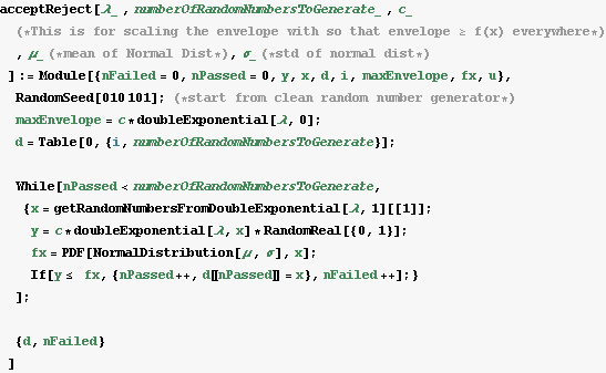
Accept Reject Algorithm Implementation

In[224]:=

Test case for n=10,000

Test the above function, and make a plot of histogram overlaid on top of density of N(0,1)

In[225]:=

Out[232]=

In[233]:=

Out[233]=

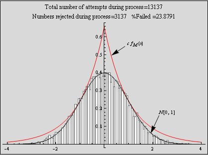
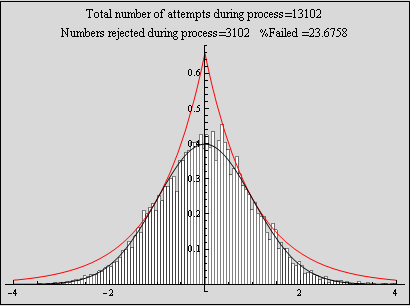
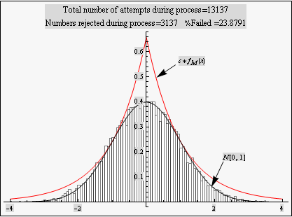
The above is a plot showing the histogram for random numbers generated using the accept - reject method for N=10,000. The random numbers are very close the N[0,1] which indicates this method is working well. The larger N is, the more closely the random numbers histogram will approach N[0,1] probability density.

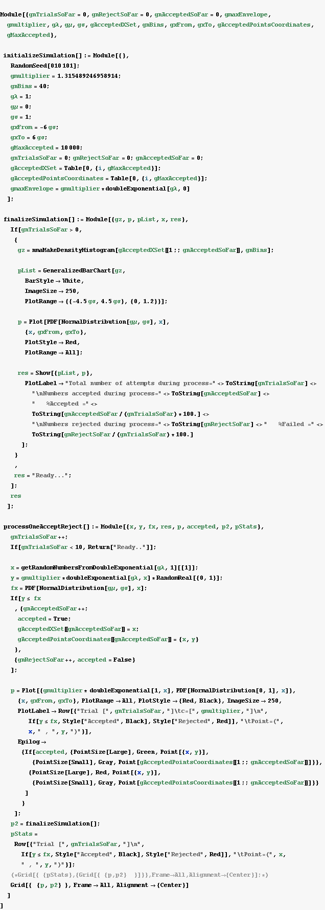
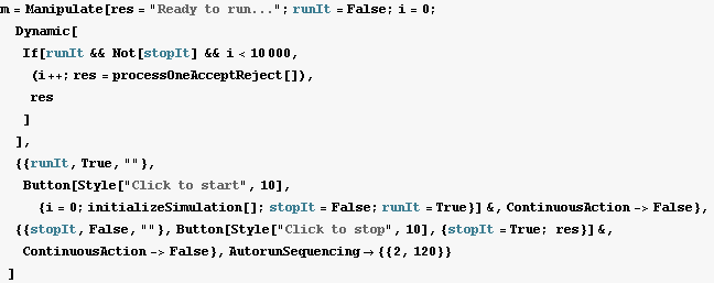
I have implemented a GUI based simulation as well for the above problem, please see the appendix below to run the simulation part.

Problem 3 simulation

In[234]:=

In[235]:=

Out[235]=

Created by Wolfram Mathematica 6.0 for Students - Personal Use Only  (25 September 2007)