Answer:
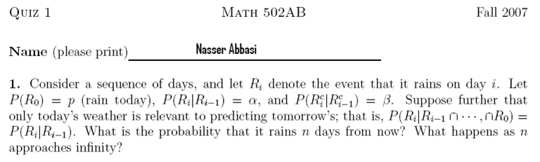
Given:
 Event that it rains on day
 ,Event that it does not rain on day
 Probability of rain on day
 ,Probability of rain on day
  given it rained on day
 ,Probability of no rain on day
  given it did not rain on day
Find:
Probability of rain in  days and what happen as
Solution:
Consider the experiment that generates today's weather. Hence possible outcomes can be divided into 2 disjoint events: rain and no rain (A day can either be rainy or not, hence this division contains all possible outcomes).
Hence

Now using the law of total probability, we write
 | (1) |
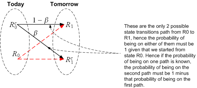
But
Note: To proof the above, we can utilize a simple state transition diagram as follows
Now, substitute (2) into (1) and given that  and
and  and
and  , then (1)
becomes
, then (1)
becomes
 | (3) |
Now we can recursively apply the above to find probability of rain on the day after tomorrow. Let
 and
and  , hence the above (1) becomes
 | (4) |
Now using (3) for  and given that
  (This probability does not change, since we are
told only today's weather is relevant), and given that
(This probability does not change, since we are
told only today's weather is relevant), and given that  and that
  ,
then (4) becomes
,
then (4) becomes

We see that as we continue with the above process, terms will be generated with the form
(something) and (something)
 , where the powers
  are getting larger and larger as
  gets
larger. But since
gets
larger. But since  , hence all these terms go to zero. So we only need to look at the terms which do not
contain a product of
, hence all these terms go to zero. So we only need to look at the terms which do not
contain a product of  and product of
Hence the above reduces

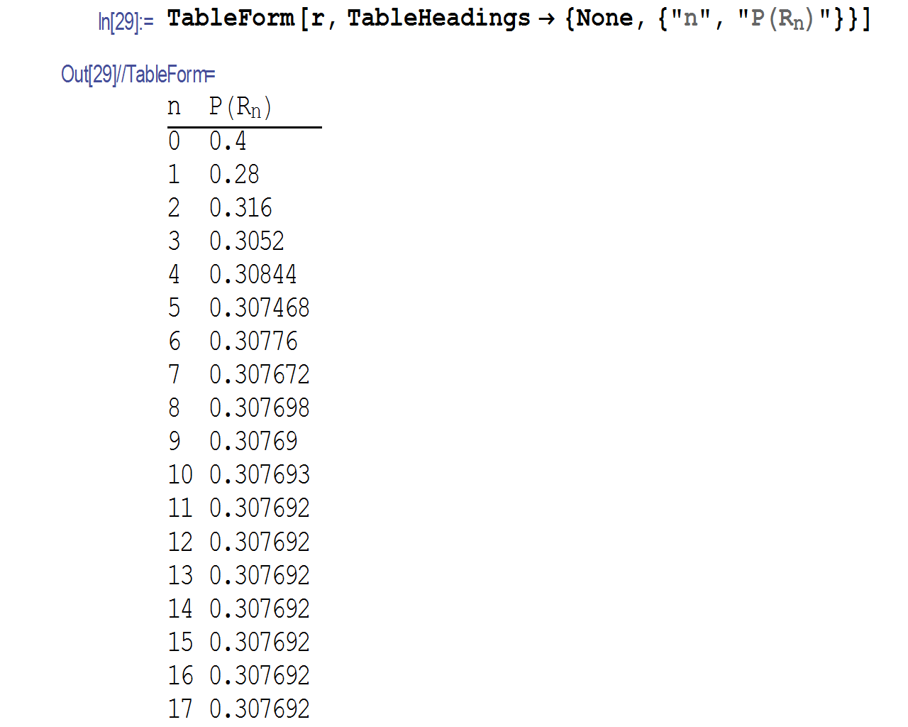
There is a pattern here, to see it more clearly, I generated more  for
for  using a small
piece of code and removed all terms of higher powers of
using a small
piece of code and removed all terms of higher powers of  as described above, and I get the following
table
as described above, and I get the following
table
 |  |
 |  |
 |  |
 |  |
 |  |
 |  |
 |  |
 |  |
Hence the pattern can be seen as the following

Where  for even
  and
and  for odd
  , and
, and  means to round to nearest lower integer
and
means to round to nearest lower integer
and  means to round upper.
The above is valid for very large  .
.
As 
 will reach a fixed value (I first though it will always go to 1, but that turned out not
to be the case). I could not find an exact expression for
will reach a fixed value (I first though it will always go to 1, but that turned out not
to be the case). I could not find an exact expression for  as
as  , but I wrote a small program
which simulates the above, and generates a table. Here is a table for few values as
, but I wrote a small program
which simulates the above, and generates a table. Here is a table for few values as  gets large, these are all
for
gets large, these are all
for  notice that
  fluctuates up and down from one day to the next as it converges
to its limit.
fluctuates up and down from one day to the next as it converges
to its limit.
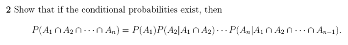
Given: Conditional probabilities exist
Show: 
Solution:
Since Conditional probabilities exist, then we know that the following is true

Let  and
and  hence the above becomes

Now apply the same idea to the last term above. In other words, we write

We repeat the process until we obtain 
Hence, putting all the above together, we write

The above is what is required to show (terms are just rewritten is reverse order from the problem statement, rearranging, we obtain

QED
Given:
Axioms of probability:

 then
then 
 are disjoint events (i.e.
  ) then

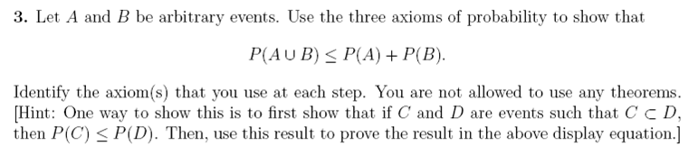
Show that 
Solution:
There are 4 possible cases.
 are disjoint


 have some common events between them. In other words
Case 1: If  are disjoint then
  by set theory. Now apply the probability operator on
both sides we obtain that
by set theory. Now apply the probability operator on
both sides we obtain that

Now, by Axiom 3,  hence the above becomes

Case 2: If  then
then  by set theory. Now apply the probability operator on both sides we
obtain that
by set theory. Now apply the probability operator on both sides we
obtain that

But  since
since  and so
  by axiom 2. Hence the above
becomes
by axiom 2. Hence the above
becomes
 | (0) |
Case 3: This is the same as case 2, just exchange  and
and 
case 4: Since, by set theory

Then apply Probability operator on both sides

But by set theory  is disjoint from
  , then by axiom 3 the above becomes
 | (1) |
Similarly, by set theory

Then apply Probability operator on both sides

But  is disjoint from
  , by set theory, then by axiom 3 the above becomes
 | (2) |
Now by set theory

Apply the probability operator on the above

But  and
and  are disjoint by set theory, then above can be written using axiom 3
as
are disjoint by set theory, then above can be written using axiom 3
as
 | (3) |
Add (1)+(2)

subtract the above from (3)

Cancel terms (Arithmetic)
![P (A ∪ B ) − [P (A ) + P (B)] = − P (B ∩ A )](q1123x.svg)
or (algebra)

Since  is an event in
  then
then  by axiom 2, hence the above can be written
as
by axiom 2, hence the above can be written
as
 | (4) |
conclusion: We have looked at all 4 possible cases, and found that  or
or
 , hence
Note: I tried, really tried, to find a method which would require me to use the hint given in the problem
that if  , then
  but I did not need to use such a relationship in the above. But I still
show a proof for this identity below
but I did not need to use such a relationship in the above. But I still
show a proof for this identity below
Given:  , Show
proof:
 by set theory
 by applying probability to each side.
But  are disjoint by set theory, hence
  by axiom 3.
Hence  , or
, or 
But by axiom 2,  , hence
  , QED
, QED

Given:  binomial r.v., i.e.
  Find the mode. This is the value
  for
which
for
which  is maximum
The mode is where  is maximum. Consider 2 terms, when
  , and
, and  , hence
  will be increasing when
But

Hence

so  is getting larger when
  or
or

So as long as  , pmf is increasing. Since
  is an integer, then we need the largest integer such
that it is
is an integer, then we need the largest integer such
that it is  , hence

Given:

members are affected independently
Find: probability 2 individuals are affected in population of size 100,000
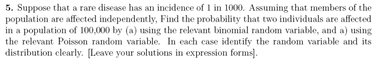
part(a)
In Binomial random variable we ask: How many are infected in a trial of length  given that the
probability of being infected in each trial to be
given that the
probability of being infected in each trial to be  Here we view each trial as testing an individual.
Consider it a 'hit' if the individual is infected. The number of trials is
Here we view each trial as testing an individual.
Consider it a 'hit' if the individual is infected. The number of trials is  , which is
  , and
, and
 .
.
Therefore,  how many are infected in population of 100000
Hence the probability of getting  hits is, using binomial r.v. is (
 in this case)

or numerically

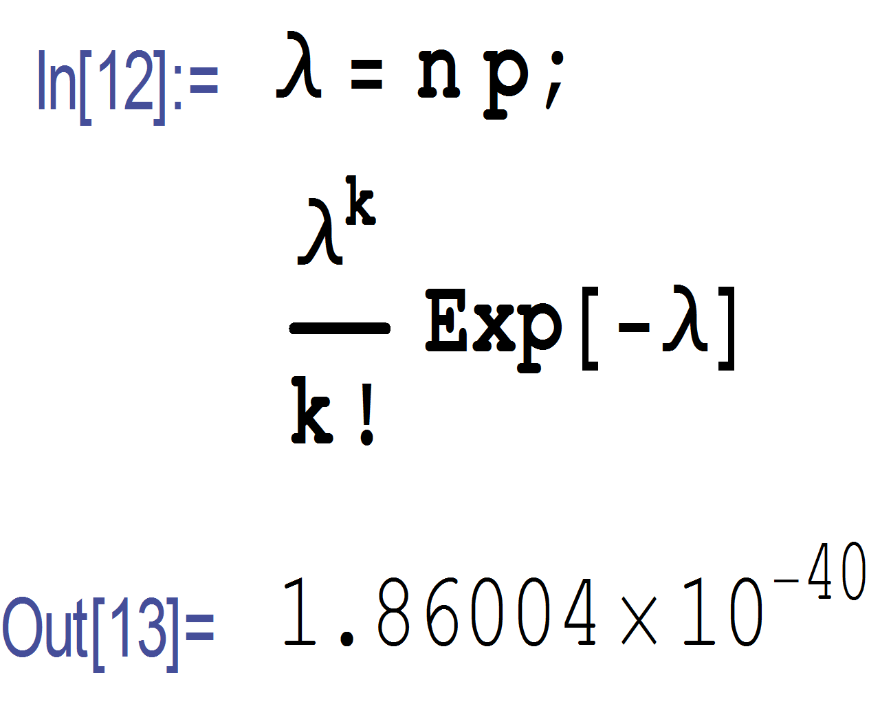
(b)Using Poisson r.v. Poisson is a generalization of Binomial. X is the number of successes in infinite number
of trials, but with the probability of success in each one trial going to zero in such a way that  .We
compute
.We
compute 

Hence here  how many are infected as
  gets very large and
  , the probability of infection in each
individual goes very small in such a way to keep
, the probability of infection in each
individual goes very small in such a way to keep  fixed at a parameter
  . Since here
  is large and
  is
small, we approximate binomial to Poisson using
is
small, we approximate binomial to Poisson using 
Hence

ps. computing a numerical value for the above, shows that using Binomial model, we obtain

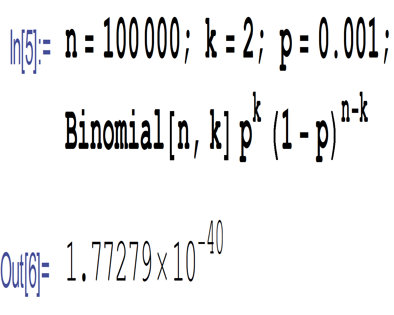
and using Poisson model
I am not sure, these are such small values, this means there is almost no chance of finding 2 individuals infected in a population of 100,000? I would have expected to see a much higher probability than the above. I do not see what I am doing wrong if anything.
