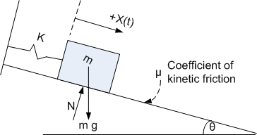
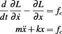
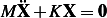
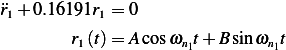
Find the equation of motion for the following system
Solution
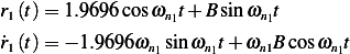
Assume initial conditions are  and
and  . Assume that
  was positive (i.e. to the right of the
static equilibrium position, and also assume that
was positive (i.e. to the right of the
static equilibrium position, and also assume that 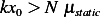 ). This second requirement is needed to
enable the mass to undergo motion by overcoming static friction. The normal force
). This second requirement is needed to
enable the mass to undergo motion by overcoming static friction. The normal force  is given
by
is given
by

And the dynamic friction force  due to the dynamic friction is defined as follows
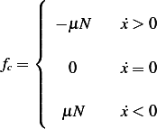
But since  , then the above becomes
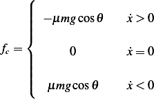 | (1) |
Where  is the coefficient of dynamic friction. Now we can obtain the Lagrangian
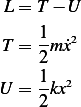
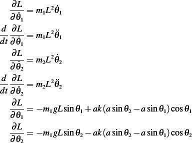
Hence
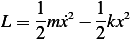
and
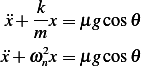
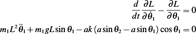
Then the EQM is
Where  is given by (1). Since
  sign depends in the mass is moving to the left or to the right, we will
generate 2 equation of motions, one for each case.
sign depends in the mass is moving to the left or to the right, we will
generate 2 equation of motions, one for each case.
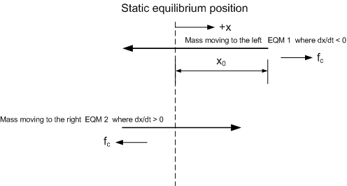
When mass is moving to the left, EQM 1 is
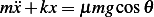 | (2) |
When mass is moving to the right, EQM 2 is
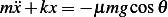 | (3) |
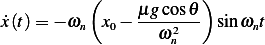
So, for the first move, starting from  and moving to the left, we have

Guess  , hence
 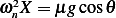 or
or  , and
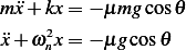
, and  , therefore, the solution to
EQM 1 is
, therefore, the solution to
EQM 1 is
 hence
hence 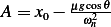 , then
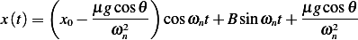
and
Hence  , then EQM is (for
  )
)
 | (4) |
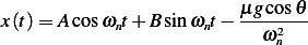
The mass will move according to the above equation (4) until the velocity is zero, then it will turn and start moving to the right. To find the time this happens:
Now solve for  when
when  , i.e.,
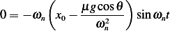 | (5) |
Hence  , where
 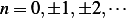 The case for
  do not apply since this implies
  , then
consider the next time this can happen, which is
, then
consider the next time this can happen, which is  , which implies
 | (6) |
Now we need to determine  at this time
  since this will become the initial
  for the second equation of
motion going to the right in the second leg of the journey. Using (4) and (6) we obtain
for the second equation of
motion going to the right in the second leg of the journey. Using (4) and (6) we obtain
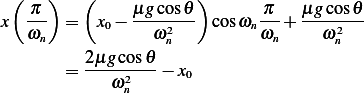
Notice that in the above equation,  is a positive number, since we assumed that the initial conditions
 was to the right of the static equilibrium position, and we are assume the right of the static
equilibrium position to be positive. This also implied that
was to the right of the static equilibrium position, and we are assume the right of the static
equilibrium position to be positive. This also implied that  will be negative number (which is
what we expect, as the mass will by the end of its first trip be on the left of the static equilibrium
position).
will be negative number (which is
what we expect, as the mass will by the end of its first trip be on the left of the static equilibrium
position).
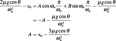
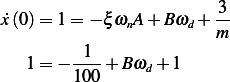
Now we can use right equation of motion (EQM 2) to solve for the mass moving to the right. Notice that
the initial conditions for this motion are 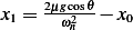 and
and 
The equation of motion is now
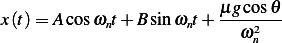
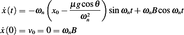
With the general solution
 | (7) |
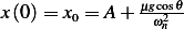
At  , hence from the above
Hence (7) becomes
And
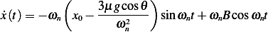
But  at
at  , hence the above becomes
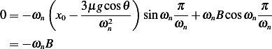
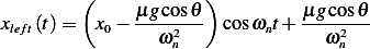
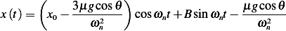
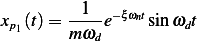
Hence  , then the EQM for the right move is, for
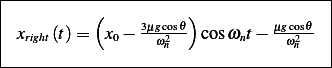
This diagram below summarize this
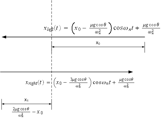
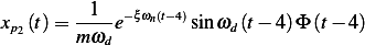
Now, we would like to have one equation to express the motion with for any time instance when the mass is moving to the left, or to the right. Looking at the above 2 equation of motion, we see immediately that we can write the equation of motion as follows
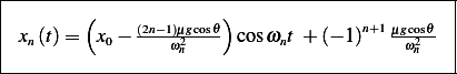
Where  above is the number of the trip. So, the first trip, going from
  and moving to the left, will have
 , and then second trip, moving from
  and going to the right will have
  , and so on. As for the
time during which trip travels, this is found by the following equation
, and so on. As for the
time during which trip travels, this is found by the following equation
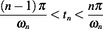
What the above is saying is that for first trip ( ), we have

And for the second trip, we have

etc...
Now that we have one equation, and we have the time during which each equation is valid, we can now
plot the equation of motion vs. time. The following is a plot for some values for  . Please see the
appendix for the Matlab code which generated this simulation.
. Please see the
appendix for the Matlab code which generated this simulation.
Observation found on this problem: Changing the angle of inclination  causes no change in results. In other
words, the same oscillation will occur for flat plane (
causes no change in results. In other
words, the same oscillation will occur for flat plane ( ) or for
  or any other angle. The
reason is because
or any other angle. The
reason is because  , the initial position, is measured from the static equilibrium position, and
this static equilibrium position will be different as the angle changes, but the effect of the angle
change is already accounted for by this change and will not be reflected in the actual displacement
, the initial position, is measured from the static equilibrium position, and
this static equilibrium position will be different as the angle changes, but the effect of the angle
change is already accounted for by this change and will not be reflected in the actual displacement
 .
.
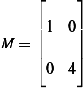
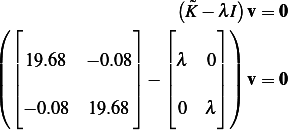
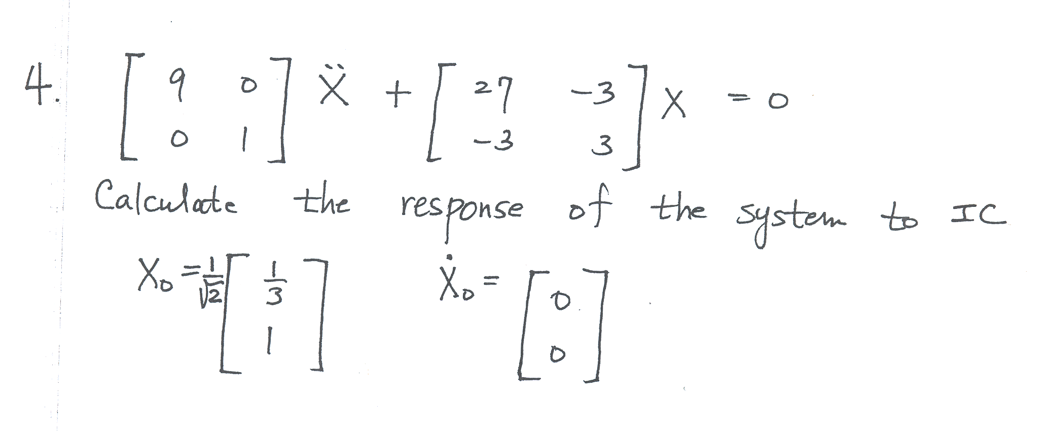
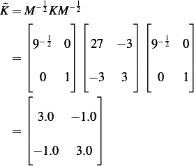
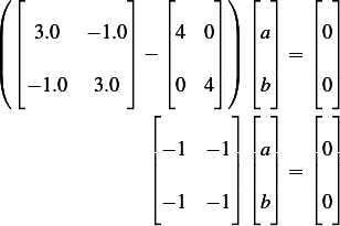
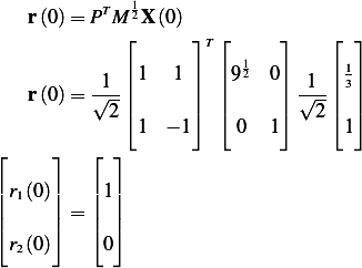
Given 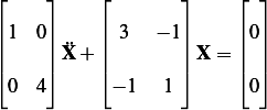 ,
,  , use modal analysis to calculate the solution of this
given
, use modal analysis to calculate the solution of this
given 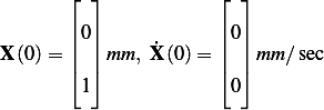 also calculate the eigenvalues of the system and the normalized
eigenvectors.
also calculate the eigenvalues of the system and the normalized
eigenvectors.
Answer
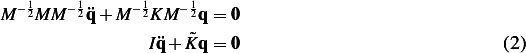
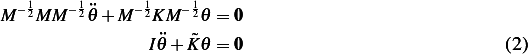
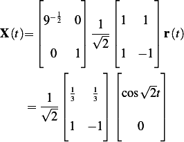
Since this is a 2 ODE's that are coupled, we use modal analysis to de-couple the system first in order to obtain 2 separate ODE's which we can then solve easily.
Let
 and let
 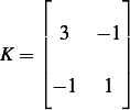 , then the above system becomes
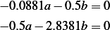
 | (1) |
Let  , then
  and the above equation becomes
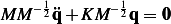
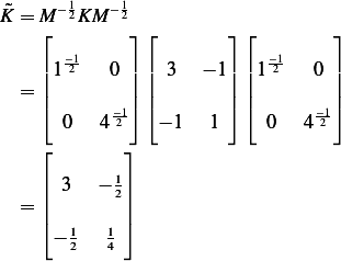
premultiply by  we obtain
Where 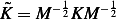
Let  , then
  and (2) becomes

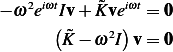
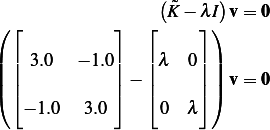
Let  then we have
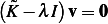 | (3) |
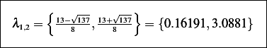
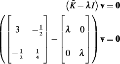
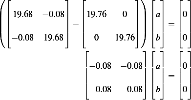
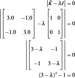
For  , we requires that
  But
But
Hence
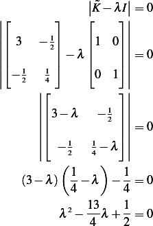
Hence
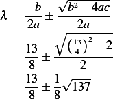
Hence
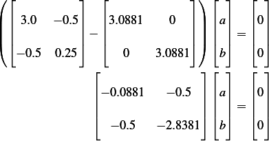
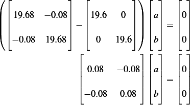
From (3) we then have
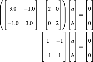
When  we obtain
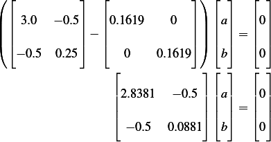
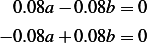
Hence
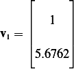
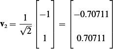
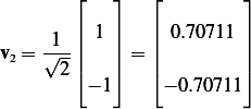
Let  , then
  , hence the second eigenvector is
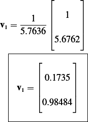
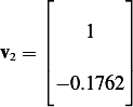
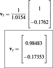
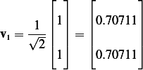
 , hence normalized
  is
is
When  we obtain
Hence
Let  in the first equation above, then
 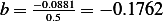 , hence the first eigenvector
is
, hence the first eigenvector
is
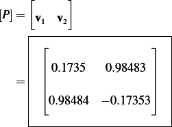
 , hence normalized
  is
is
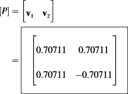
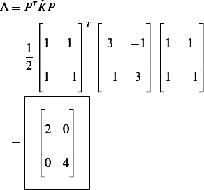
Then the  matrix
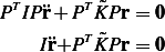
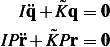
Now let  then equation (2) above becomes

Premultiply by 
Let  then the above becomes
 | (4) |
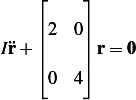
Now find 
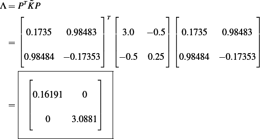
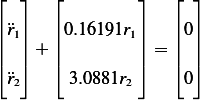
 Hence (4) becomes
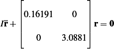
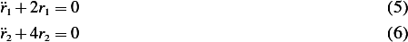
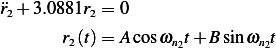
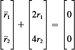
Which can be written as 2 equations
or
With IC given as
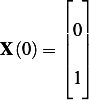
and
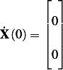
Now  and
and  , hence
  , then
now need to find  but since
  , then
  as well.
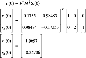
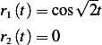
Now we can solve for  and
and  since we have the IC. From (5) above
At 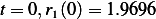 , hence
  , then
At 
Hence  , then
But  , hence
Similarly we find 
At  , hence
  , then
At 
Hence  , then
But  , hence
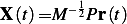
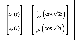
Now that we found the solution in the  space, we switch back to the original
  space
space

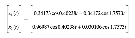
Then
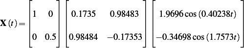

 Hence
Hence
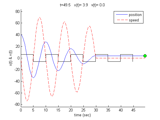
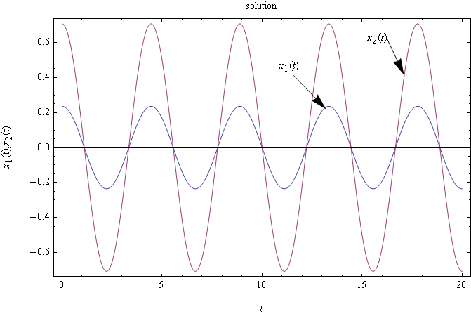
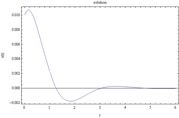
This is a plot of the solutions
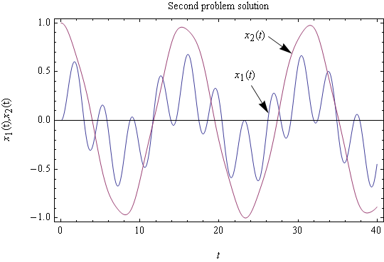
Observation on final result: Notice that power of the harmonic  rad/sec. in the motion
  is small
(amplitude is only
is small
(amplitude is only  ) hence the dominant harmonic present in
  is
is  rad/sec. and this
reflects in the plot where it appears that
rad/sec. and this
reflects in the plot where it appears that  contain one harmonic. In the case of
  we see from the
solution that both frequencies contribute equal amount of power, hence the plot for
we see from the
solution that both frequencies contribute equal amount of power, hence the plot for  reflects
this.
reflects
this.

Solution Use as generalized coordinates  ,. Assume that the spring remain horizontal, and assume that

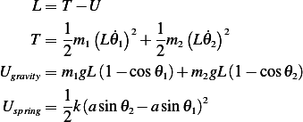
Hence

Now determine the Lagrangian equation
Hence the EQM for  is
is
Now apply small angle approximation.  and
and  hence
hence
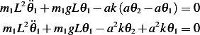
 | (1) |
And the EQM for  is
is

Now apply small angle approximation.  and
and  hence
hence
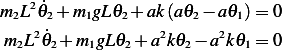
Therefore
 |
Now we write the system as 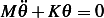
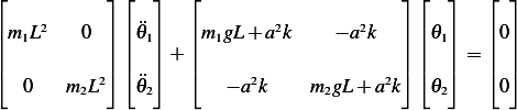
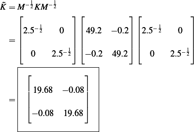
Substitute numerical values for the above quantities, we obtain
The above can be written as

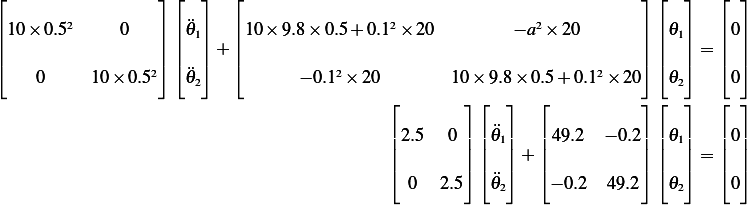
Let  , then
  and the above equation becomes
premultiply by  we obtain
Where 
Let  , then
  and (2) becomes
Let  then we have
 | (3) |
For  , we requires that
  But
But
Hence
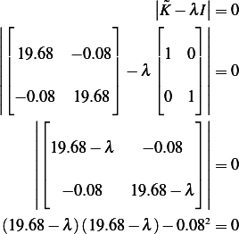
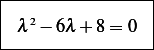
Hence the characteristic equation is
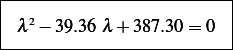
Hence
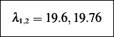
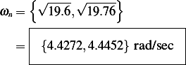
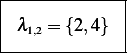
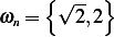
Hence the natural frequencies are
From (3) we then have
When 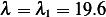 we obtain
Hence
Hence  then
then

When 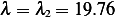 we obtain
Hence  , then
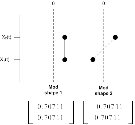
Now that we have obtained the eigenvectors of the de-coupled system, we can plot the mode shapes2 . I will use a diagram similar to that shown in the textbook Engineering Vibration by Inman on page 313)

Where 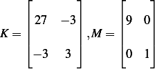 Let
Let  , then
  and the above equation
becomes
and the above equation
becomes

premultiply by  we obtain
Where 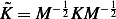
Let  , then
  and (2) becomes
Let  then we have
 | (3) |
For  , we requires that
  But
But
Hence
Hence the characteristic equation is
Hence
Then the natural frequencies are
From (3) we then have
When  we obtain
Hence

Then  , hence
When  we obtain
Hence  , then
Then the matrix
Now let  then equation (2) above becomes
Premultiply by 

Let  then the above becomes
 | (4) |
Now find 
Hence (4) becomes
Which can be written as 2 equations
or
With IC given as 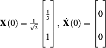 , but
, but
 and
and  , hence
  , then
And since  , then
  , now we have found IC for
  we can solve the ODEs
 hence
hence  , and
, and  , similarly,
  , and
, and  , hence
But
Then
Hence
Here is a plot of the solution
 , hence
  rad/sec and
  , hence the system is
underdamped and
, hence the system is
underdamped and  rad/sec
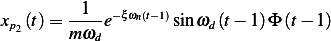
Let the response to  be
be  and let the response to
  be
be  hence the response of the
system becomes
hence the response of the
system becomes
 | (1) |
Where
 | (2) |
And
 | (3) |
and

Hence, substitute (2),(3) into (1)
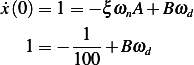
Now using IC to find  . Note, we use only
  for the purpose of finding
  from
I.C's since the response to the delayed impulse is not active at
from
I.C's since the response to the delayed impulse is not active at  . We find
And for the derivative
Hence
Hence

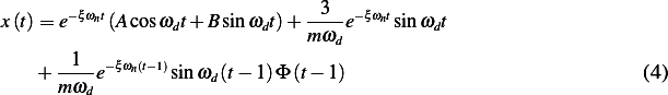
Therefore the solution is, by substituting values found for  into the general solution from above
equation (4), we obtain
into the general solution from above
equation (4), we obtain
 | (5) |
The following is a plot of the solution for up to 
 , hence
  rad/sec and
  , hence the system is
underdamped and
, hence the system is
underdamped and  rad/sec
Let the response to  be
be  and let the response to
  be
be  hence the response of the
system becomes
hence the response of the
system becomes
 | (1) |
Where
 | (2) |
And
 | (3) |
and
To find  use only
  At
At  . We find
And for the derivative

Hence
Hence

Therefore the solution is, by substituting values found for  into the general solution from above
equation (4), we obtain
into the general solution from above
equation (4), we obtain
 | (5) |
The following is a plot of the solution for up to 
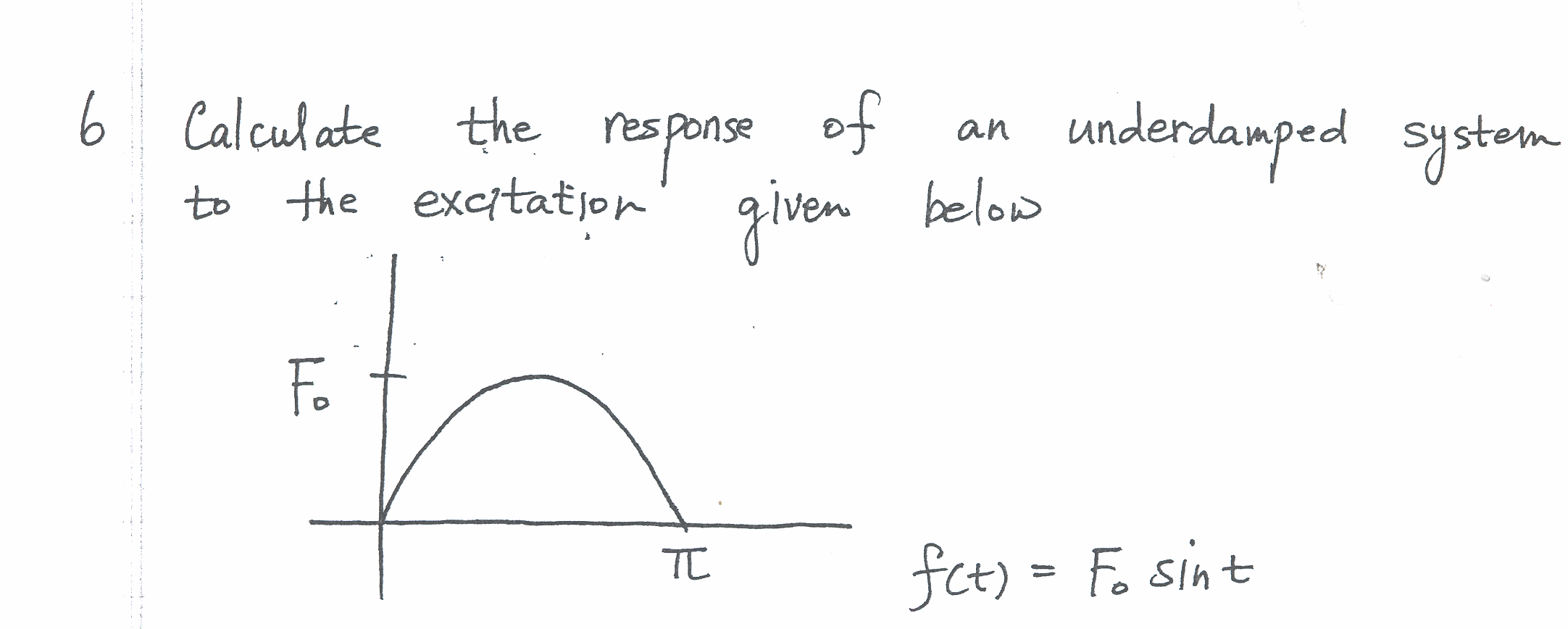
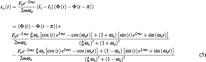
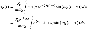
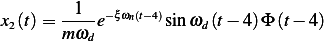
Let the response by  . Hence
 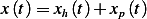 , where
  is the particular solution, which is the
response due the the above forcing function. Using convolution
is the particular solution, which is the
response due the the above forcing function. Using convolution
Where  is the unit impulse response of a second order underdamped system which is
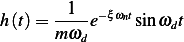
hence
Using ![1
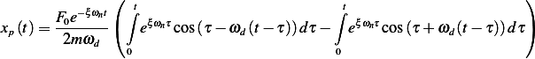
sin Asin B= 2[cos (A − B)− cos(A +B )]](ME354x.png) then
then
![1
sin(τ)sin(ωd(t− τ))= --[cos(τ − ωd(t− τ))− cos(τ+ ωd(t− τ))]
2](ME355x.png)
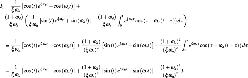
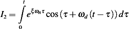
Then the integral becomes
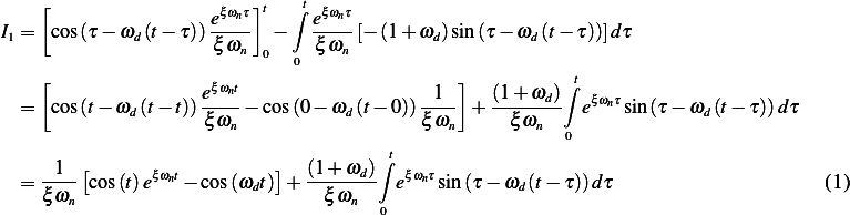
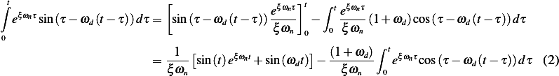
Consider the first integral  where
where
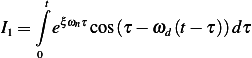
Integrate by parts, where  , Let
, Let  and let
 , hence
Integrate by parts again the last integral above, where  , Let
, Let  and
let
and
let  , hence
Substitute (2) into (1) we obtain
Hence
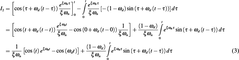
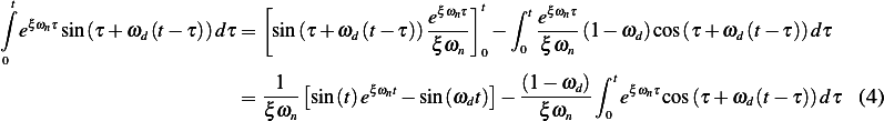
Now consider the second integral  where
where
Integrate by parts, where  , Let
, Let  and let
 , hence
Integrate by parts again the last integral above, where  , Let
, Let  and
let
and
let  , hence
Substitute (4) into (3) we obtain
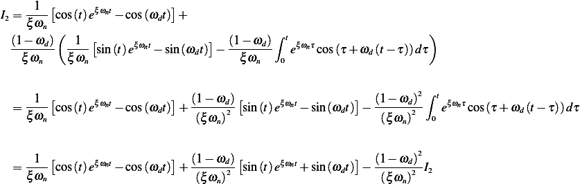
Hence
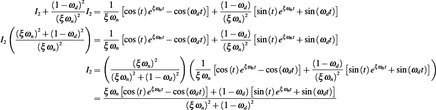
Using the above expressions for  , we find (and multiplying the solution by
  since
the force is only active from
since
the force is only active from  to
to  , we obtain
Hence 

And

Hence the overall solution is

The above solution is a bit long due to integration by parts. I will not solve the same problem using Laplace transformation method. The differential equation is

Take Laplace transform, we obtain (assuming  and
and  )
)
Now we find Laplace transform of 
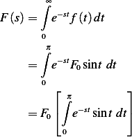
Integration by parts gives
![[1 + e−πs]
F (s)= F0 -----2-
1 + s](ME396x.png) | (8) |
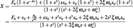
Substitute (8) into (7) we obtain
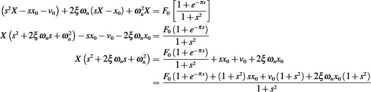
Hence
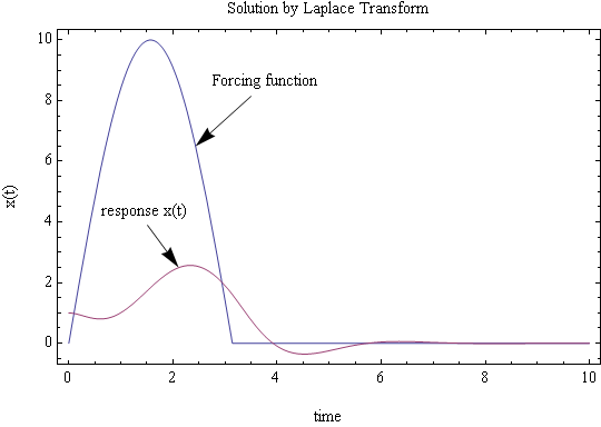
Now we can use inverse Laplace transform on the above. It is easier to do partial fraction decomposition
and use tables. I used CAS to do this and this is the result. I plot the solution  . I used the following
values to be able to obtain a plot
. I used the following
values to be able to obtain a plot 
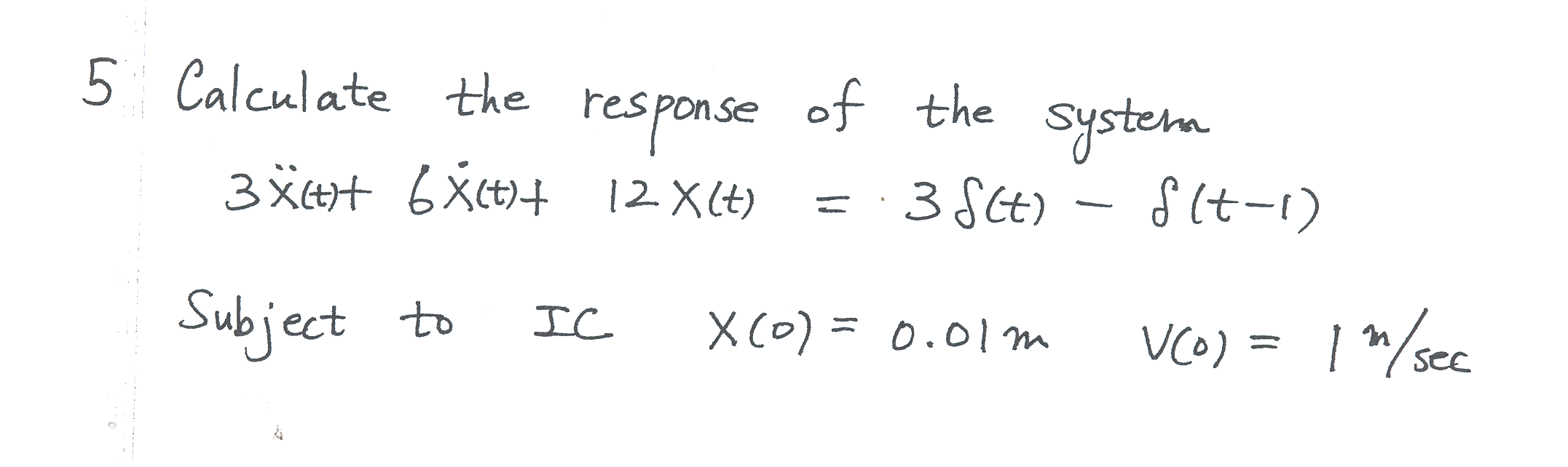
Problem
Solve  with the IC's
Answer
 , hence
  rad/sec and
  , hence the system is
underdamped and
, hence the system is
underdamped and  rad/sec
Let the response to  be
be  and let the response to
  be
be  hence the response of the
system becomes
hence the response of the
system becomes
 | (1) |
Where
 | (1) |
And
 | (3) |
and
Hence, substitute (2),(3) ,(4) into (1)
 | (4) |
Now using IC to find 

and
At  Hence the above becomes (terms with
  and
and  vanish at
  by
definition)
by
definition)
Hence (1) becomes

If we substitute the numerical values for the problem parameters, the above becomes
Compare the above with the solution given in class, which is
Problem
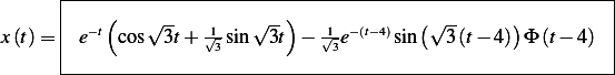
Solve  with the IC's
Answer
 , hence
  rad/sec and
  , hence the system is
underdamped and
, hence the system is
underdamped and  rad/sec
Let the response to  be
be  and let the response to
  be
be  hence the response of the
system becomes
hence the response of the
system becomes
 | (1) |
Where
 | (1) |
And
 | (3) |
and
Hence, substitute (2),(3) ,(4) into (1)
 | (4) |
Now using IC to find 

Hence

Now take the derivative of the above and evaluate at zero to find  . In doing so, we need to consider
only the
. In doing so, we need to consider
only the  . The reason is that the particular solution
  of the delayed pulse (the second
pulse) will have no effect at
of the delayed pulse (the second
pulse) will have no effect at  and the first pulse particular solution
  will also have
no contribution, since its response is assume to occur at
will also have
no contribution, since its response is assume to occur at  , i.e. an infitismal time after
  .
Therefore, since we intend to evaluate
.
Therefore, since we intend to evaluate  at
at  , we only need to take
  derivative at this
point
derivative at this
point

At  Hence the above becomes
Hence (1) becomes

If we substitute the numerical values for the problem parameters, the above becomes
Which now matches the solution given in class