Math 503 computing assignment 1
FEM and FDM solution for u''(x)+q u(x)=f
by Nasser Abbasi
Project for Mathematics 503, Summer 2007. California State University, Fullerton, CA.
In this project we are asked to implement the Finite Element Methods (FEM) and Finite difference method (FDM) to find the solution u(x) for the following differential equation, and also compare both methods.
![]()
The 2 methods are compared for speed of convergence to the exact solution. The exact analytical solution is known for this simple differential equation:
![]()

![]()
![]()
![]()
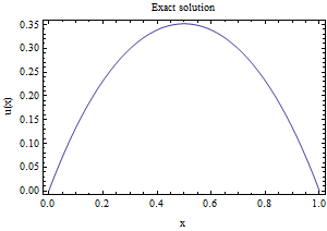
The numerical solution for u(x) at each grid point is compared to the true solution, then the maximum error using each method is found. Also the RMSerror is calculated.
A brief overview of the FEM and FDM scheme used is now discussed.
For the FEM, the variational approach is used (as contrasted by the Garlkin method). In the variational method, we seek to find a solution y(x) to a functional J(y(x)) defined by an integral such that this solution y(x) minimizes this functional. This solution will be the solution to the differential equation itself. However, we do not use nor try to find the differential equation at all in this method. We work directly on the first variation equation J'(y;φ)=0 itself by finding y(x) such that J'(y;φ)=0 for all the ![]() permissible directions. In the Garlkin method, we are given the differential equation, and then we substitute equation (2) below into the differential equation itself.
permissible directions. In the Garlkin method, we are given the differential equation, and then we substitute equation (2) below into the differential equation itself.
In this problem the φ functions are also the basis for the vector space in which the solution y(x) defined in. In other words, these ![]() represent a basis for the V space of y(x) and we seek a solution
represent a basis for the V space of y(x) and we seek a solution
![]()
Which satisfies ![]() for all the basis functions
for all the basis functions ![]() .
. ![]() is defined by
is defined by
![]()
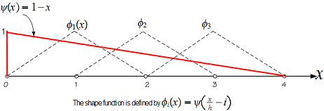
Where i is the shape function number i=1,2,3..n and ψ(x)=1-x for 0<x<1, and ψ(x) = 0 for x>1 and ψ(x)=ψ(-x). The relationship between ![]() and ψ(x) is illustrated in this diagram
and ψ(x) is illustrated in this diagram
In this problem the functional we want to minimize is given
![]()
Where q>0 and f are given constants. In the first part of this project we found that J(u) achieves a minimum iff J'(y;φ)=0 where J' (y; φ) is given by
![]()
We start the FEM by setting up the equations J' (y; ![]() ) =0, therefore, we will have N number of equations, where N is the number of the shape functions φ. Hence for each
) =0, therefore, we will have N number of equations, where N is the number of the shape functions φ. Hence for each ![]() shape function
shape function ![]() we would have
we would have

The above will generate N algebraic equations which we will then solve for the ![]() coefficients. Once the
coefficients. Once the ![]() is found then we can determine the FEM solution u(x) from (2) above at any x.
is found then we can determine the FEM solution u(x) from (2) above at any x.
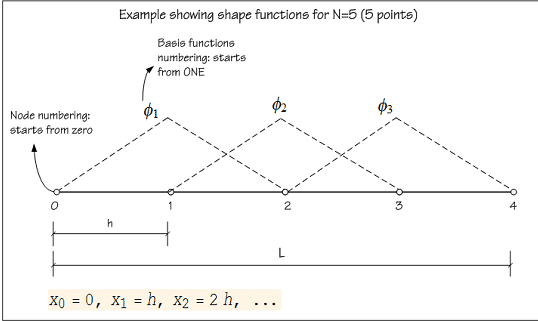
It is important to agree on the numbering scheme of nodes, elements, and shape functions. The following diagram illustrates the numbering used.
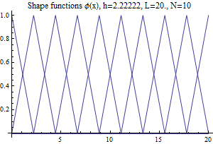
This below plots the shape functions for illustration.

When generating each equation ![]() for each basis
for each basis ![]() we take advantage of the domain of influence of each specific
we take advantage of the domain of influence of each specific ![]() , we see from above that
, we see from above that ![]() is nonzero only over the range
is nonzero only over the range ![]() . The program calls a function to generate one equation for each basis. This function performs the integration shown in equation (4) but will only do the integration over
. The program calls a function to generate one equation for each basis. This function performs the integration shown in equation (4) but will only do the integration over ![]() since
since ![]() =0 elsewhere.
=0 elsewhere.
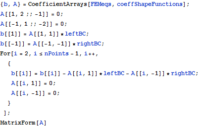
Once the N equations are computed, We solve Ax=b to find x where x here is the vector which contain ![]() coefficients as shown in equation (2) above. The matrix A will be tridiagonal in this problem since for each basis
coefficients as shown in equation (2) above. The matrix A will be tridiagonal in this problem since for each basis ![]() (other than the first and the last basis) we see that it overlaps with 2 other basis
(other than the first and the last basis) we see that it overlaps with 2 other basis ![]() and
and ![]() hence this causes an equation with 3 unknowns to be generated (
hence this causes an equation with 3 unknowns to be generated (![]() . This below is an small function will shows the equations for N=8 and shows the A matrix to make this point more clear.
. This below is an small function will shows the equations for N=8 and shows the A matrix to make this point more clear.

| -5.71429+4.15952 c[1]+1.55476 c[2]==0 |
| -11.4286+1.55476 c[1]+8.31905 c[2]+1.55476 c[3]==0 |
| -11.4286+1.55476 c[2]+8.31905 c[3]+1.55476 c[4]==0 |
| -11.4286+1.55476 c[3]+8.31905 c[4]+1.55476 c[5]==0 |
| -11.4286+1.55476 c[4]+8.31905 c[5]+1.55476 c[6]==0 |
| -11.4286+1.55476 c[5]+8.31905 c[6]+1.55476 c[7]==0 |
| -11.4286+1.55476 c[6]+8.31905 c[7]+1.55476 c[8]==0 |
| -5.71429+1.55476 c[7]+4.15952 c[8]==0 |
Which in Ax = b format, the above becomes

The above shows that A is diagonally dominant, and tridiagonal. Hence a tridiagonal solver is used since it is much faster than Gaussian elimination in this case. In FEM, the generate A matrix will always contain diagonal bands as the above and these matrices are sparse in nature.
In the FDM method, the central difference method is used to approximate u''(x). Hence in this method we already know the differential equation and we work directly on the differential equation, while in the FDM method above, we do not know necessarily what the differential equation is and work directly on the first variational term.
The central difference scheme is given by

Where ![]() means u at grid point
means u at grid point ![]() . Now we substitute the above equation directly into the differential equation -u'' (x) + q u(x) = f and obtain
. Now we substitute the above equation directly into the differential equation -u'' (x) + q u(x) = f and obtain
![]()
![]()
Hence for each point (we start from the first internal grid point i=1 and not from the boundary point i=0) and hence for each such internal point, we see that we have 3 unknown. Hence the general Ax=b equations will also be tridiagonal. This is illustrate by this short example below. Notice that 2 equations are inserted manually into the set of the generated equations since ![]() and
and ![]() , since these are boundary conditions given.
, since these are boundary conditions given.

| 4 u[2]-0.1225 (u[1]-2 u[2]+u[3])==4 |
| 4 u[3]-0.1225 (u[2]-2 u[3]+u[4])==4 |
| 4 u[4]-0.1225 (u[3]-2 u[4]+u[5])==4 |
| 4 u[5]-0.1225 (u[4]-2 u[5]+u[6])==4 |
| 4 u[6]-0.1225 (u[5]-2 u[6]+u[7])==4 |
| 4 u[7]-0.1225 (u[6]-2 u[7]+u[8])==4 |
| u[1]==0 |
| u[8]==0 |
This shows the A matrix from the above set of equations. We see it is a tridiagonal, The last 2 rows are for the 2 equations for the boundary conditions
![]()

The error in approximation between numerical and exact solution for u(x) as a function of increasing number of points is generated for up to n=200 and the complete table is shown in the appendix at the end of the report. Both max error and RMS error is calculated for each n. Below is partial listing of the table for number of points n=4..21

| number of elements | FEM rms error | FDM rms error | FEM max error | FDM max error |
| 2 | 0.242315 | 0.228426 | 0.726946 | 0.685279 |
| 3 | 0.22625 | 0.22037 | 0.639932 | 0.6233 |
| 4 | 0.20898 | 0.205904 | 0.709175 | 0.698885 |
| 5 | 0.194493 | 0.192655 | 0.681121 | 0.674754 |
| 6 | 0.182459 | 0.18126 | 0.706204 | 0.701634 |
| 7 | 0.172336 | 0.171503 | 0.692309 | 0.689007 |
| 8 | 0.163691 | 0.163085 | 0.705185 | 0.702615 |
| 9 | 0.156207 | 0.15575 | 0.696893 | 0.694883 |
| 10 | 0.149652 | 0.149297 | 0.704718 | 0.703072 |
| 11 | 0.14385 | 0.143568 | 0.69921 | 0.697859 |
| 12 | 0.138669 | 0.138441 | 0.704464 | 0.703322 |
| 13 | 0.134007 | 0.133819 | 0.700541 | 0.699572 |
| 14 | 0.129783 | 0.129626 | 0.704312 | 0.703473 |
| 15 | 0.125933 | 0.1258 | 0.701375 | 0.700647 |
| 16 | 0.122405 | 0.122291 | 0.704213 | 0.703571 |
| 17 | 0.119156 | 0.119058 | 0.701933 | 0.701365 |
| 18 | 0.116153 | 0.116068 | 0.704146 | 0.703638 |
| 19 | 0.113365 | 0.11329 | 0.702323 | 0.701869 |
| 20 | 0.110768 | 0.110702 | 0.704097 | 0.703686 |
The numerical results in the table is also plotted. The following 2 plots compare both methods accuracy for max error and rms error as function of increasing n for n up to 200. The full table is in the appendix.

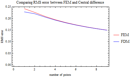

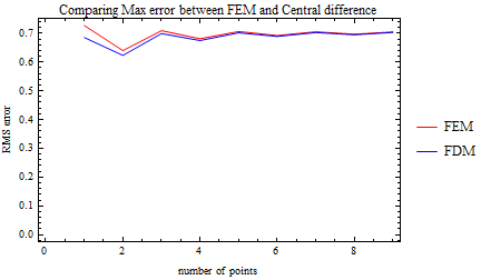
The FDM is more accurate than the FEM for low N. Two error measurements were used: RMS error and Max error. For low N, FDM is more accurate than FEM, even more so when looking at the RMS error as seen by the plot above.
From the plots above we observe that as N increases both methods become as accurate as each others in approximating the exact solution. This happens for both max error and for RMS error.
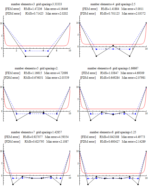
The following diagram below shows this more clearly, where both FEM and FDM solution are plotted for n=2,3,4,5,6,7,8. We see that FDM for low N is more accurate, but FEM catches up very quickly, and about N=8 FEM max error was the same as FDM error for up to 6 decimal places. The following was done for L=10 instead of L=1 to make the plots a little more interesting.

FEM method is more complicated to implement than FDM. And from the above, we see that it does not give more accurate results than the simpler FDM method using central difference scheme. One might ask then why use FEM over FDM? Although this did not come up in this project, one can argue the following advantages of one method over the other:
FEM solution u(x) can be used at point x in the domain and not just at the grid points ![]() as with FDM
as with FDM
FEM can handle complicated boundary geometry, while FDM requires simple boundary geometry.
With FEM, one can add more elements in the vicinity where the solution changes rapidly to obtain more accuracy there. With FDM this is normally not done. Although one can also implement adaptive grid sizing as well in FDM, it is normally done in the time domain and not in the space domain.
Does not require knowing the differential equation to find the solution when working from the Variational approach as in this project. FDM requires knowing the differential equation.
More accurate than FEM for low N. This is in particular when the exact solution is not too smooth. When the solution is not too smooth, more points are needed to make FEM as accurate as FDM.
Simpler to code and implement.
Global parameters

Function name: makeEquation and its helpers
Input: the shape function number. Also access variable ![]() to generate the weak form equation for the
to generate the weak form equation for the ![]() shape function
shape function
Purpose: generate the weak for equation for ![]() shape function. To make it simpler, I have 2 special functions to handle the first and last shape elements since these are special conditions.
shape function. To make it simpler, I have 2 special functions to handle the first and last shape elements since these are special conditions.
Returns: The weak for equation for the ![]() shape function
shape function

Function name: φ
Input: i, the shape function number. z, the distance along the domain to find φ at
Purpose: generate the φ function.
Returns: the value of φ function at this z value.
![]()

Function name: yApprox
Input: x, distance along x direction. coeff, the ![]() coefficient found for the FEM approximation from the equation y=
coefficient found for the FEM approximation from the equation y=![]() , h is the grid spacing, nPoints is number of points.
, h is the grid spacing, nPoints is number of points.
Purpose: calculate the solution from the FEM calculation after the ![]() has been found.
has been found.
Returns: u(x) based on FEM approximation

Function name: getUCentralMethod
Input: access to number of points
Purpose: performs finite difference calculation using the central difference scheme for the second derivative.
Returns: data, which is a matrix of 2 columns. The first column is the x value, second column is the u value at this x.
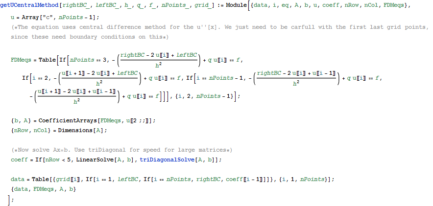
Function name: getErrorsInApproximation
Input: access FEM matrix, grid points, FDM data.
Purpose: called to calculate the RMS error and Max error for the FEM and FDM methods.
Returns: 4 numbers. rmserrorFEM, maxErrorFEM, rmserrorDiff, maxErrorFDM
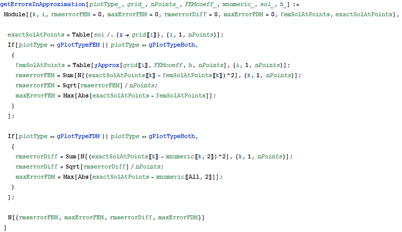
Function name: triDiagonalSolve
Input: A,d
Purpose: called to solve for x in Ax=d for use on tridiagonal matrices A. This only works correctly if A is diagonally dominant.
Returns: vector x, the solution from Ax=d
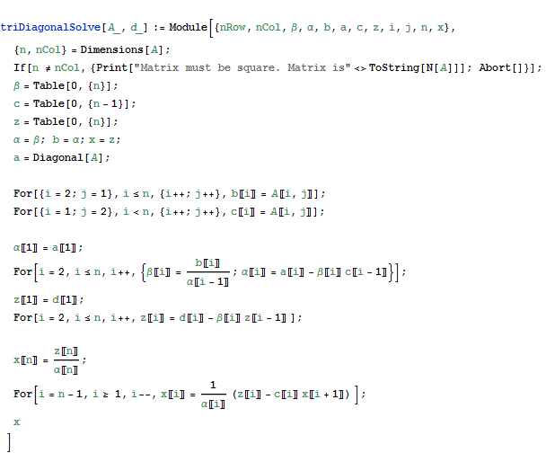
Function name: process
Input: access to all the input parameters from the GUI. See init[] function above.
Purpose: called by the GUI after the call to init[] is made. This function is the driver which calls all the other functions above. It find the FEM and FDM solutions and plot them.
Returns: Graphics plot for the GUI to display
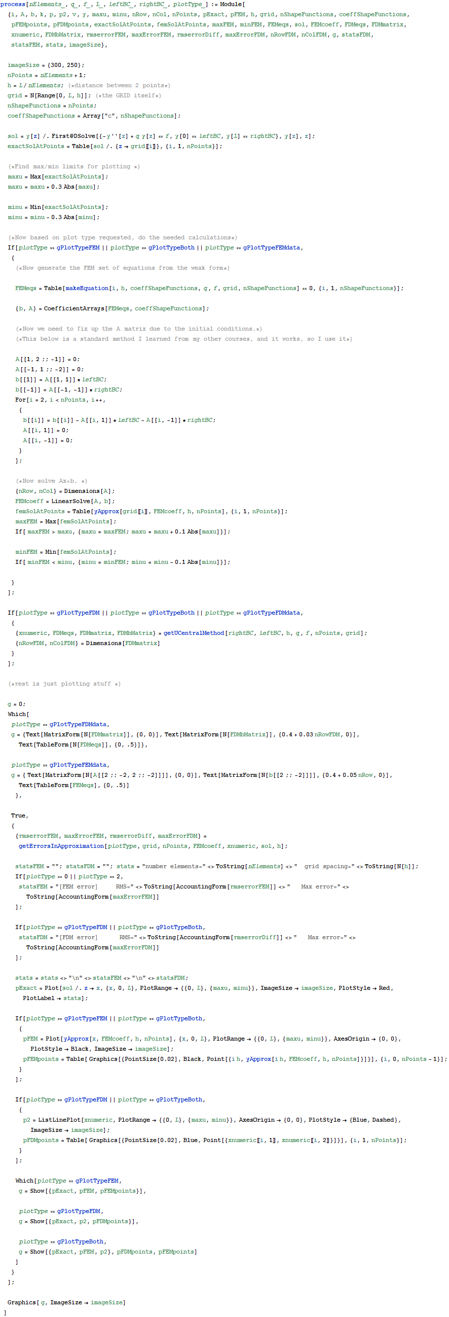
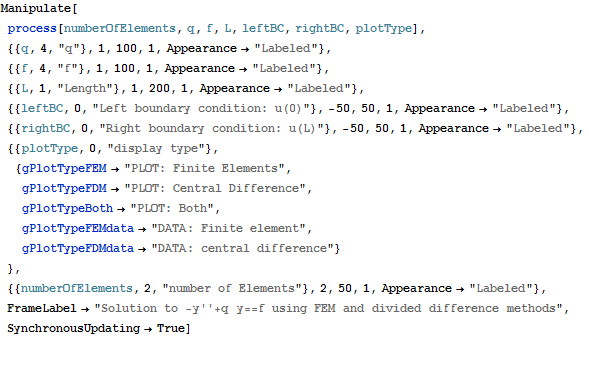
This is the Manipulate function. This is the GUI interface for the program. It display the GUI and called the Init and Process functions above to do the actual calculations
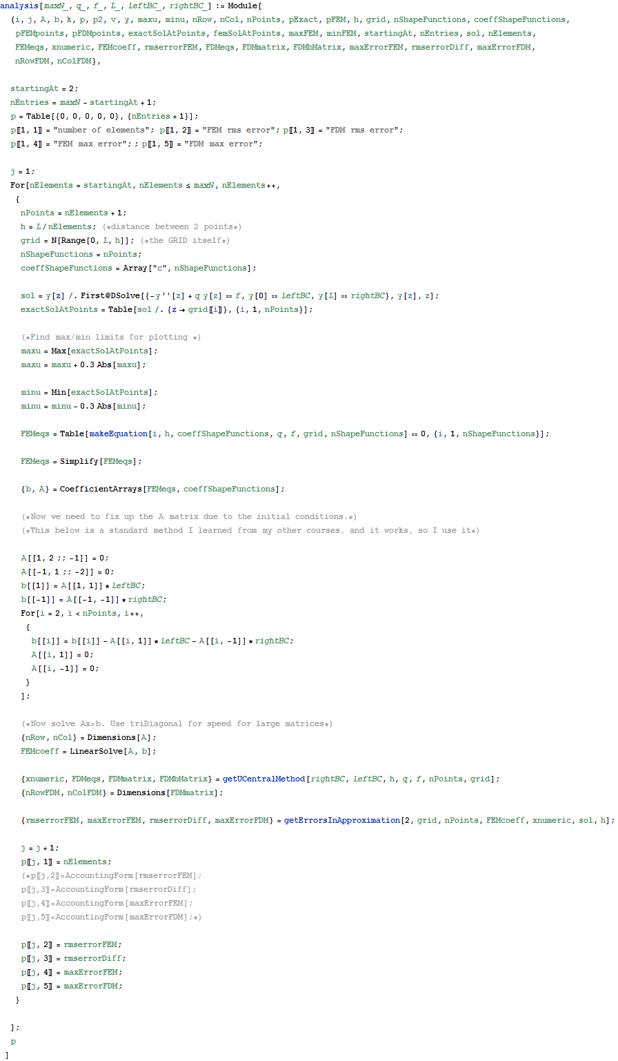
This is an analysis function. Not part of the main program. It is used to generate a table that shows the error (RMS and Max) between FEM and FDM methods as n, the number of points, is increased.

| number of elements | FEM rms error | FDM rms error | FEM max error | FDM max error |
| 2 | 2.48355 | 0.672655 | 7.45065 | 2.01796 |
| 3 | 1.47236 | 0.71425 | 4.16446 | 2.0202 |
| 4 | 1.41884 | 0.701125 | 5.0011 | 2.03572 |
| 5 | 1.16615 | 0.676051 | 4.72098 | 2.05559 |
| 6 | 1.03847 | 0.649284 | 4.69309 | 2.07981 |
| 7 | 0.927077 | 0.623795 | 4.59354 | 2.1087 |
| 8 | 0.842188 | 0.600427 | 4.49773 | 2.14289 |
| 9 | 0.772973 | 0.579316 | 4.39248 | 2.18321 |