HW3, MAE 200A. Fall 2005. UCI
Nasser Abbasi
Due: Oct. 13 at beginning of class
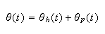
Analyze the forced response of the pendulum. The forcing, as demonstrated in class, is the sinusoidal side to side movement of the attachment point.
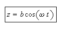
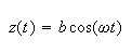
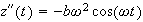
Assume the lateral motion of the attachment point is of the form
 is the maximum displacement. The linearized dynamics about the equilibrium at
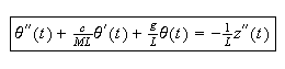
 are
are
Construct a physical pendulum. It can be as simple as the one I used in class,
although a rigid rod would be preferable to an elastic one. Estimate the
values of
 ,
,
 and
and
 and use these values in your calculations.
 = length of the rod;
 = mass of the pendulum bob;
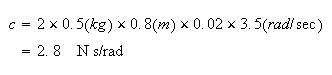
 =damping coefficient
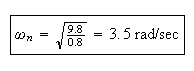
Determine the natural frequency
 and
damping ratio
and
damping ratio
 of
your pendulum.
of
your pendulum.
Determine the general solution (homogeneous plus particular) for the linear pendulum model. You can use the result I gave in lecture if you know how to obtain it. If you don't know how to obtain it, this would be a good opportunity to learn how to.
Using the particular solution, construct the Bode plots theta (amplitude and
phase angle as functions of the forcing frequency
 ).
).
Experiment with forcing your pendulum at different frequencies and convince yourself that what you see corresponds to the predictions from the Bode plots.
If you move the attachment point according to
 where,
relative to the natural frequency
where,
relative to the natural frequency
 of the pendulum,
 is much less than
 ,
,
 is close to
 ,
and
,
and
 is greater than
 ,
describe qualitatively what the
,
describe qualitatively what the
 response will look like after the homogeneous solution has died out. Your
answer should be based on theory not experiment.
response will look like after the homogeneous solution has died out. Your
answer should be based on theory not experiment.
Please turn in all your work except for your pendulum. Bring your pendulum to class if you want to show it off, but this is optional.
A simple pendulum was used for this experiment.
The Mass
 was weighted and found out to be about

The length
 was measured to be 80 cm or

To determine the damping coefficient, since
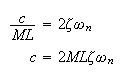 I will
first find
I will
first find
 .
.
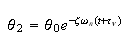
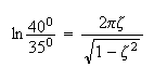
The method of logarithmic decrement was used. The logarithmic decrement
 is the natural logarithm of the ratio of any two successive amplitudes in the
same direction. The pendulum mass is held initially at an angle
is the natural logarithm of the ratio of any two successive amplitudes in the
same direction. The pendulum mass is held initially at an angle
 in the positive direction, and then released. The mass will then make one full
cycle by swinging to left and then back to the same side as it started and
stop before starting its second cycle and so on. The angle the mass reach at
the end of its first cycle was estimated to be
in the positive direction, and then released. The mass will then make one full
cycle by swinging to left and then back to the same side as it started and
stop before starting its second cycle and so on. The angle the mass reach at
the end of its first cycle was estimated to be
 and the angle it reached at the end of it second full cycle was estimated to
be
and the angle it reached at the end of it second full cycle was estimated to
be

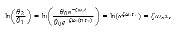
Hence
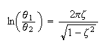
The following diagram showing the process and the derivation of the above equation
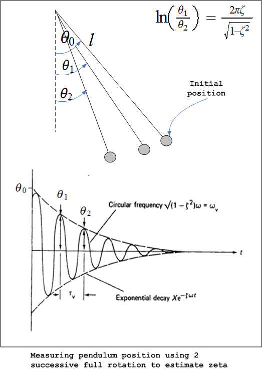
To derive the
equation We
utilize the above plot of
We
utilize the above plot of
 for a damped second order system.
In the above diagram
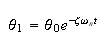 and
and
 where
where
 is the time it takes to make one full swing between these 2 successive
oscillations.
is the time it takes to make one full swing between these 2 successive
oscillations.
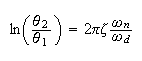
But
 where
where
 is the damped natural frequency. Hence
 hence
hence
But
 hence the above equation becomes

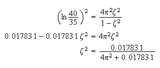
Now that this equation is derived, it can be used to estimate
 ,
Once
,
Once
 is found then
 can be easily found.
square each side and solve for


Next, since
 Hence,
then
Hence,
then
and since
 ,
then
,
then
First we find an analytical solution
 .
.
where
 is the homogenous solution (due to initial conditions) and
 is the particular solution (due to the forcing function). To find
 ,
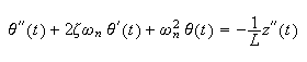
looking at the ODE
,
looking at the ODE
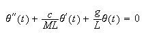
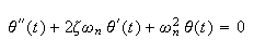
We see this is a standard second order system. Let
 ,
,
 ,
hence we can write the above as
,
hence we can write the above as
 the
solution is
the
solution is
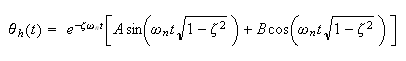
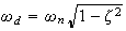
where the damped natural frequency be
 hence the above can be written as
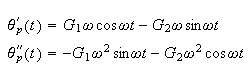
Now we can find the particular solution. Since the forcing function is a
sinusoidal, we can try
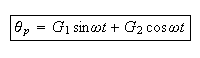
This particular solution will take care of the case when the forcing function
is out of phase with the response, that is why both a
 and a
and a
 function are present. Substitute
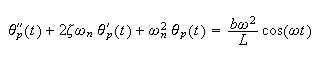
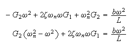
 into the dynamic equation that represents the linearized pendulum given by
and since
 then
then
 hence the above equation becomes
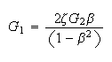
Now
Hence (4) becomes
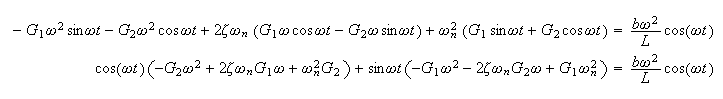
compare coefficients of
 we get
and
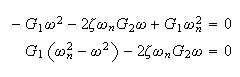
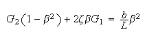
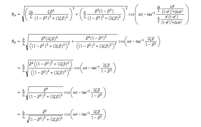
Need to solve (5) and (6) for
 first divide (5) and (6) by
 and call the ratio
 which is the response ratio, to obtain new expressions for
 and (6)
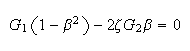
from (6a)
Plug (7) into (5a) we obtain
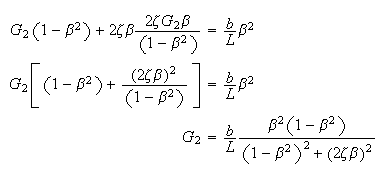
Substitute (8) into (7) to solve for

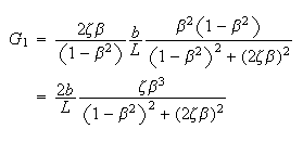
Hence
Where
 are as given above. Hence
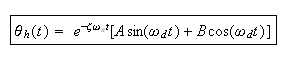
Hence the general solution
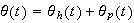 is
is
Where
 ,
can now be determined from initial conditions. However, since we are
interested in steady state solution (not the transient solution), we do not
need to find these constants for the purpose of this solution.
,
can now be determined from initial conditions. However, since we are
interested in steady state solution (not the transient solution), we do not
need to find these constants for the purpose of this solution.
The first term in the solution (the
 )
term, will damp down quickly with time since it has the inverse exponential
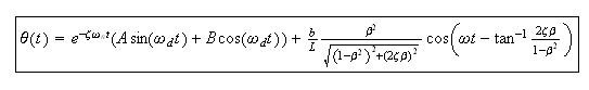
term in it. What is left then is the particular
solution.
)
term, will damp down quickly with time since it has the inverse exponential
term in it. What is left then is the particular
solution.
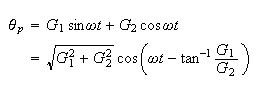
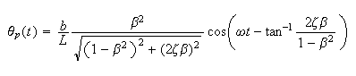
Since
Hence in the above equation we can write it as
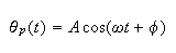
Where amplitude
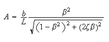 and phase
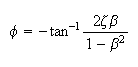
To make amplitude in degrees instead of radians, convert the above by
multiplying by

and
 ,
,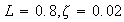 ,
and for let
,
and for let
 meters.
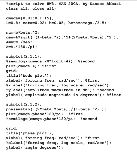
Now we are ready to generate the needed plots. I will show the following plot
where the x-axis will show the input frequency
 in rad/sec, and the y-axis will show the amplitude
 in angles.
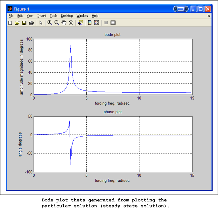
Now I changed the forcing frequency to be close to the natural frequency of the pendulum (3.5 radians per second), and observed largest oscillation at that frequency. (note: input force is lateral, at the joint, so input frequency needs to be converted from cycles per second to radiance per second).
This is in agreement with the above plot.
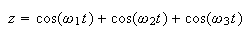
Now assume

For a linear system, the total response will be the same as the sum of the response to each of the above signals individually. (at each instance of time).
In addition, the response will have the same frequency but different amplitude and phase.
Hence the steady state amplitude will be the sum of the individual amplitudes, and the steady state phase shift will be the sum of the individual phase shifts. (at each instance of time).
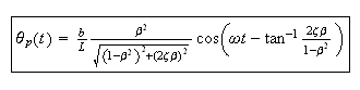
This can be answered by looking at the analytical solution found above for
 (steady state solution) and taking the limit of
 as it approaches
 or
or
 or
or
 and see what happens to the amplitude and the phase in each case.
Since we found
Where

Hence for the case when
 ,
then
,
then
 ,
hence the limit of the solution will be
,
hence the limit of the solution will be
 ,
i.e. in stead state, the displacement goes to zero. For the phase we see that
the phase
,
i.e. in stead state, the displacement goes to zero. For the phase we see that
the phase
 will also go to zero, hence response will be in-phase with the input.
For the case when
 ,
then we see
,
then we see
 becomes very large. We see that the phase term goes to zero since it goes like
 in the limit. Hence the response in steady state when the input frequency is
much larger than
in the limit. Hence the response in steady state when the input frequency is
much larger than
 will be in phase. To see what happens to the amplitude, take the limit of the
amplitude as
will be in phase. To see what happens to the amplitude, take the limit of the
amplitude as

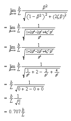
So when forcing frequency is much larger than
 ,
the steady state response will be fixed and will be proportional to the
maximum amplitude
,
the steady state response will be fixed and will be proportional to the
maximum amplitude
 .
This agrees with the plot shown above where we see the response is steady at
large
.
This agrees with the plot shown above where we see the response is steady at
large
 For the phase we see that the phase
 will also go to zero, hence response will be in-phase with the input. This
agrees with the phase plot shown.
will also go to zero, hence response will be in-phase with the input. This
agrees with the phase plot shown.
For the case when
 ,
then
,
then
 ,
hence
,
hence
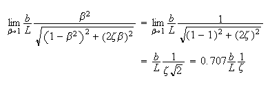
Hence the smaller the damping ratio
 ,
the larger the amplitude. This means the smaller the damping coefficient
,
the larger the amplitude. This means the smaller the damping coefficient
 the larger the amplitude. This is called resonance. For the phase, we see that
 hence at resonance, the phase is
90
hence at resonance, the phase is
90 from the input. This agrees with the plot shown.