
HW4, MAE 200A. Fall 2005. UCI
Nasser Abbasi
Compare the integration of the standard linear, constant coefficient second-order system between the 3 methods: analytic integration, Euler integration, and the Matlab integrator ODE45.
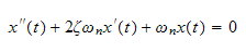
The ODE, using the derivative notation I used for the previous assignment, is
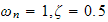
where
 is natural frequency and
 is damping ratio.
On the course website I have posted 2 m-files that you can use, or you can write your own. If you use mine, please figure out what each step does so that you can learn how to use Matlab and eventually be capable of writing your own programs. The 2 m-files, called HW4mfile and f_hw4 work together.
The first is the main program and it calls the other. You run the main program using the 'save and run' command or click on the icon. When it works it will produce Figure 1 with superimposed plots of the solutions determined in the 3 ways.
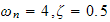
Consider three sets of system parameter values

 and
and
 (the values in the files on the website)

 and
and


 and
and


The report you turn in should include the following
Problem statement
Give good and bad numerical integrator parameters (e.g., the step size
 for the Euler integrator) and a figure illustrating good integration and a
figure illustrating bad integration. For the 'good' integration try to use a
step size that gives an accurate answer, but isn't excessively small, so that
the computational burden is minimized.
for the Euler integrator) and a figure illustrating good integration and a
figure illustrating bad integration. For the 'good' integration try to use a
step size that gives an accurate answer, but isn't excessively small, so that
the computational burden is minimized.
Describe how you adjusted the step size for the Euler integration and the
relative and absolute errors for ODE45 to get solutions that match well with
the analytic solution. How do these adjustments depend on the parameters of
the system,
 and
and
 ?
?
If you didn't have an analytic solution, which will be the case for most nonlinear ODEs, how would you know when you have an accurate numerical solution?
Please see above for the problem statement.
I start by solving the 2nd order ODE to determine the analytical solution.
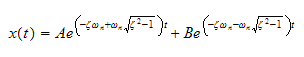
Let the solution be

Substitute in the above equation we get the characteristic equation
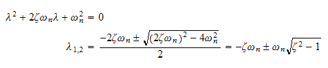
Hence the solution is
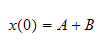
Let initial conditions be
 and
and

Hence at
 eq (1) becomes
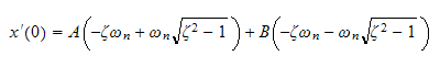
Take derivative of (1) we get
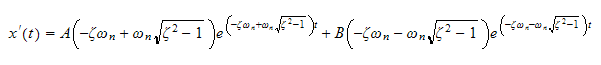
at
 the above becomes
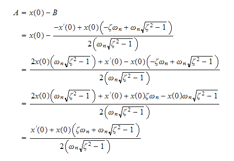
Now solve (2) and (3) for A,B. From (2)
 ,
plug into (3) we get
,
plug into (3) we get
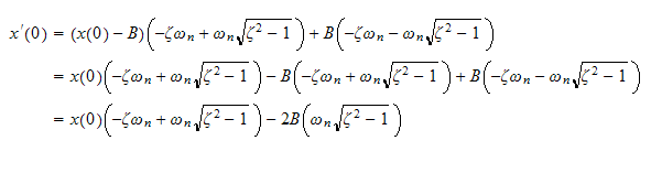
Hence
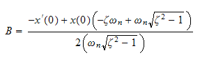
Hence from (2) we obtain

Let
 hence
hence
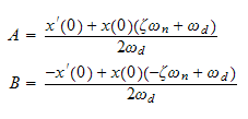
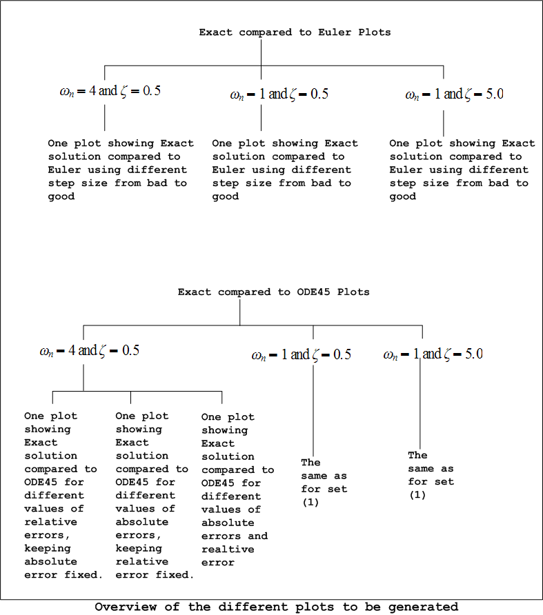
Now that we have the full analytical solution we can implement the Euler integration and compare with the analytical solution. This will be done for the 3 sets of values given. For each set try a good and a bad Euler step. The following diagram describes the types of plots that will be generated
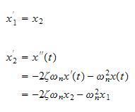
To obtain the numerical solution using the Euler method, we start by converting the 2nd order ODE to a set of 2 first order ODE as follows.
Let

Hence one state variable is the position and the second state variable is the speed.
Differentiate we obtain
We are given the initial position
 and the initial speed
 .
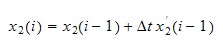
Hence to find to the position at the next time instance (i.e. to integrate
.
Hence to find to the position at the next time instance (i.e. to integrate
 )
we write
)
we write
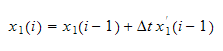
But
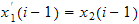 hence the above becomes
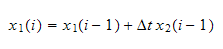
Similarly, to integrate the state variable
 we write
But
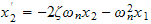 hence the above becomes
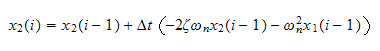
Hence equation (4) and (5) gives us the needed equation to determine the
solution (which is
 )
)
We start the process by finding
 from eq(4) in terms of
 and
and
 which are the initial conditions. Next we find
 in terms of
 and
and
 which are the initial conditions.
Next we find
 from eq(4) in terms of
 and
and
 and we again update
 to find
 .
.
This process continues until the end of the time span.
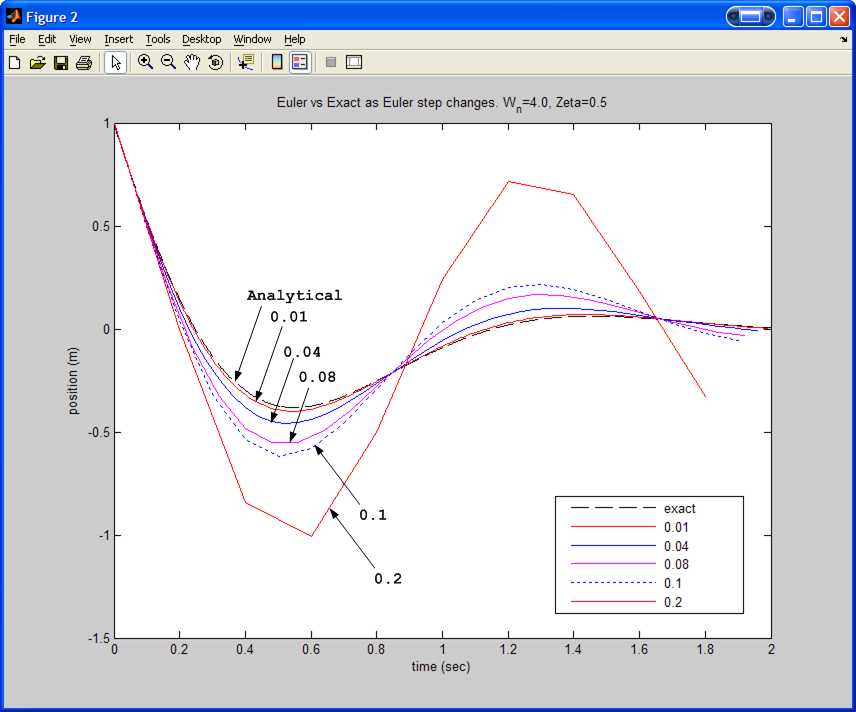
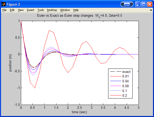
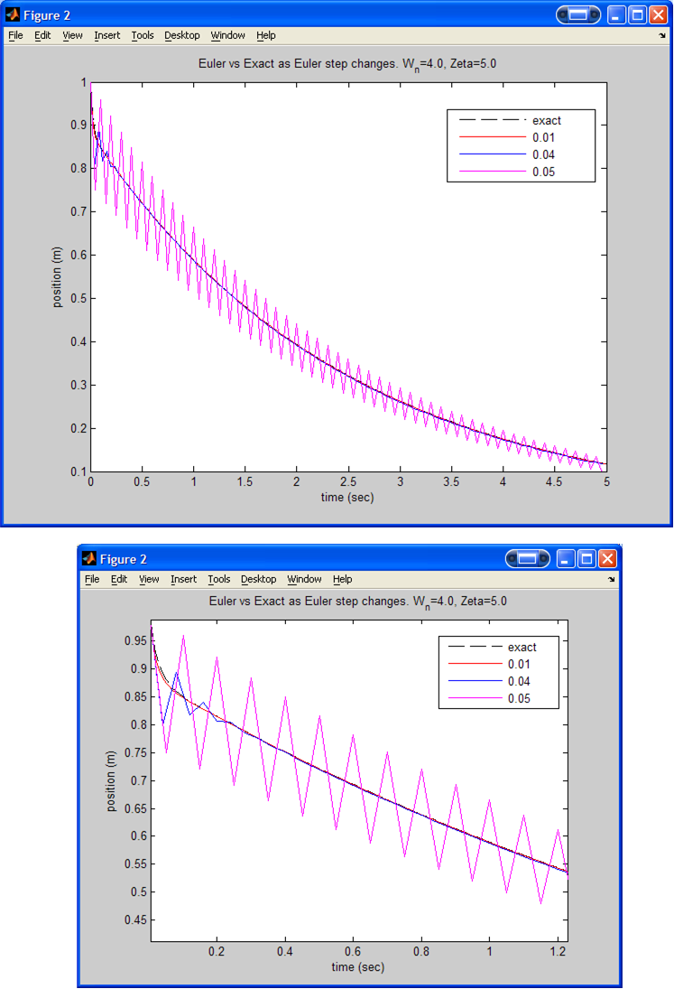
These 3 plots below show the effect of changing the Euler step. Euler step was
changed from good value (0.01) to bad value (1.2) by incrementing it and
observing how the Euler starts to produce solutions that are further and
further away from the analytical solution. Each plot was generated for
different set of values of
 and
and

Results for
 (for both small run time and longer run time).
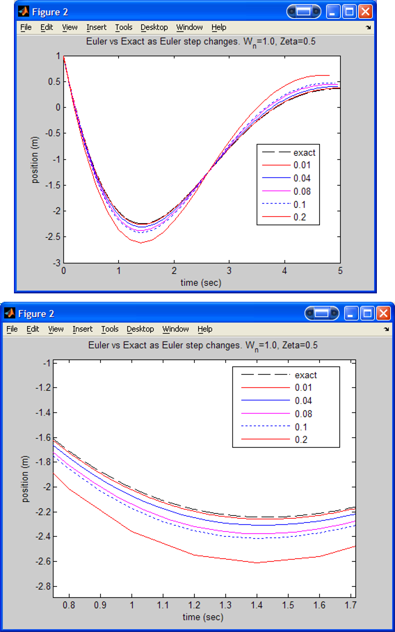
Results for
 .
(With a zoom in to better illustrate the effect of changing Euler step).
.
(With a zoom in to better illustrate the effect of changing Euler step).
Results for
 .
(With a zoom in to better illustrate the effect of changing Euler step). This
plot was done only for Euler steps of 0.01, 0.04 and 0.05.
.
(With a zoom in to better illustrate the effect of changing Euler step). This
plot was done only for Euler steps of 0.01, 0.04 and 0.05.
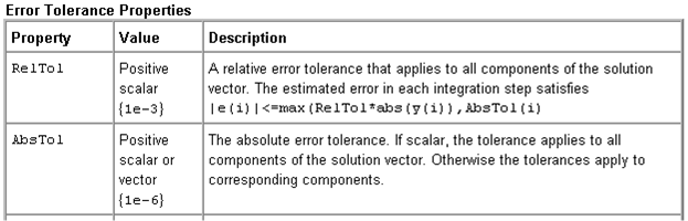
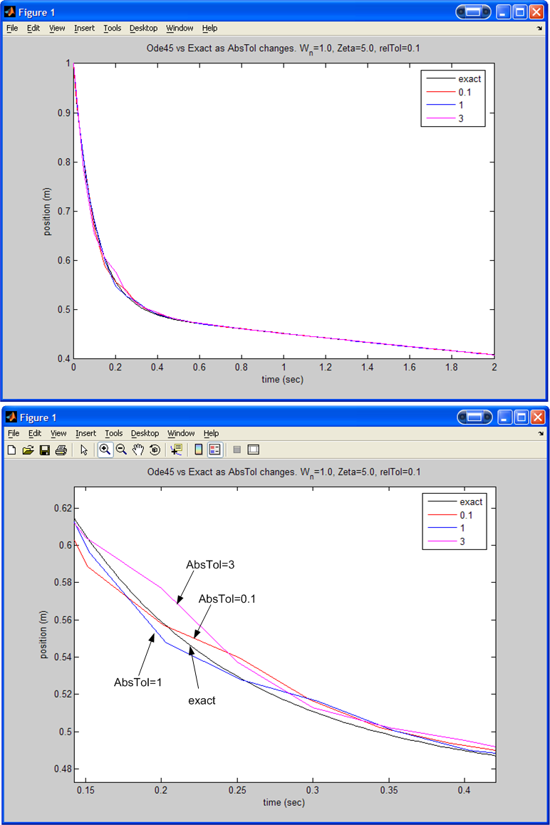
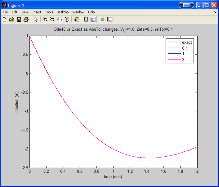
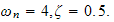
Now we compare the ODE45 Matlab numerical solution with the analytical solution. This is done for different values of relative and absolute error. These parameters are defined as follows (this is from Matlab help)
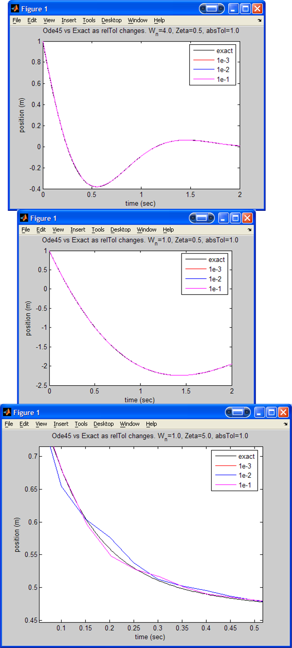
Conclusion: When the relative tolerance is made larger (while ABS. tolerance
is fixed), the solution generate by ode45 was worst. In addition, as
 increased, the solution generated by ode45 became even worst for the same
relative tolerance used. (while
increased, the solution generated by ode45 became even worst for the same
relative tolerance used. (while
 is kept fixed) i.e. Relative tolerance is sensitive to the value of

As
 is increased (while keeping everything else fixed), ODE45 solution started to
become less accurate compare to the analytical solution. Hence to improve the
ODE45 solution the absolute tolerance was decreased. Decreasing the absolute
tolerance in this case had better result on the accuracy of the solution as
compared to decreasing the relative error while keeping the absolute error
fixed.
is increased (while keeping everything else fixed), ODE45 solution started to
become less accurate compare to the analytical solution. Hence to improve the
ODE45 solution the absolute tolerance was decreased. Decreasing the absolute
tolerance in this case had better result on the accuracy of the solution as
compared to decreasing the relative error while keeping the absolute error
fixed.
The absolute and relative tolerance values were adjust by using the Matlab function odeset.
Below are few plots showing the effect of changing the absolute and relative tolerance.
First, fix relative tolerance at 0.1 and solve for absolute tolerance for values 0.01,0.1,1 and 10.
Results for
 (With a zoom in to better illustrate the effect of changing ABS. Tolerance)
Results for
 (With a zoom in to better illustrate the effect of changing ABS. Tolerance).
For this case there is almost no difference as the ABS. tolerance is changed.
Results for
 Again as above, we observe little effect on ode45 solution in this case as
ABS. tolerance is changed.
Again as above, we observe little effect on ode45 solution in this case as
ABS. tolerance is changed.
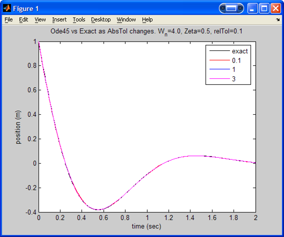
Now we repeat the above plots but we fix the ABS. tolerance to 1 and modify the relative tolerance. Use values of 1e-3, 1e-2 and 1e-1.
If you didn't have an analytic solution, which will be the case for most nonlinear ODEs, how would you know when you have an accurate numerical solution?
If the solution converges to a steady solution as the time step is decreased, then we are more confident that an accurate solution was reached.
For example, in the case of Euler numerical solution, we have only one parameter at our disposal that we can modify, which is the step size. Hence we can decrease this step size until the solution no longer changes in any significantly measure. If the solution kept changing as the step size changed, this is an indication that we have not reached the correct solution yet.