
And with 3 different loading arrangements
The deflection curve of the beam due to the loads, and the bending moment and the shear force diagrams are generated.
One can modify loadings, support conditions and other parameters such as Young's modulus (E) and the moment of inertia (I) and then observe the effect of these changes on the beam's deflection, moment and shear diagrams.
The beam deflection is normally found by solving the  order Euler Bernoulli beam differential
equation using the appropriate boundary conditions. In this demonstration, the shear force diagram is
used as the starting point and then integrated
order Euler Bernoulli beam differential
equation using the appropriate boundary conditions. In this demonstration, the shear force diagram is
used as the starting point and then integrated  times to obtain the deflection
  . The
UnitStep function was used to facilitate writing the shear force and the bending moment
equations.
. The
UnitStep function was used to facilitate writing the shear force and the bending moment
equations.
The reactions at the supports are obtained by solving the equilibrium equations for the determinate beam cases, these are the simply supported at both ends, and the cantilever cases. For the indeterminate cases (fixed at both ends, and fixed at one end and simply supported at the other end), the slope boundary conditions were used to obtain the additional equations needed to solve for all the unknown reactions.
The support conditions for the beam are first selected. There are 4 different support conditions available to choose from. The diagram near the top left corner assists one to determine this selection. The beam length is selected using the length slider located below this diagram.
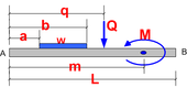
The loadings are selected by using the controls on the left side of the demonstration. A diagram is included which describes the different dimensions used to define the loading positions and the geometry.
Using this diagram with the corresponding control variables, one can define different loading configurations.
3 different load types are supported: point load  with units of force, distributed load
  with units
of force per unit length and a couple
with units
of force per unit length and a couple  with units of force times length.
Young's modulus  is selected from either the slider or by directly choosing the material from the
pop-up menu. The numbers shown for the values of E in this menu selection are the actual numerical
values for E for the material being selected. The first number is in imperial units (
is selected from either the slider or by directly choosing the material from the
pop-up menu. The numbers shown for the values of E in this menu selection are the actual numerical
values for E for the material being selected. The first number is in imperial units ( psi) and the
second number is in metric units (
psi) and the
second number is in metric units ( Pa).
Pa).
These values are obtained from standard materials reference. When using the slider to select E, each
value, internally, will be multiplied by  before being used. For example, to select a material whose E
is
before being used. For example, to select a material whose E
is  psi, set the slider at
  .
.
The moment of inertia  is selected using the slider or by defining the geometry of the beam cross
section. Only rectangular cross section is supported. When using the cross section option, the moment of
inertia is calculated using the standard formula
is selected using the slider or by defining the geometry of the beam cross
section. Only rectangular cross section is supported. When using the cross section option, the moment of
inertia is calculated using the standard formula  .
.
The amount of deflection  the beam will experience is limited to a fixed value controlled
by the parameter (D) labeled ”deflection ratio” located at the lower left part of the control
area. This parameter is defined as follows: A deflection ratio of
the beam will experience is limited to a fixed value controlled
by the parameter (D) labeled ”deflection ratio” located at the lower left part of the control
area. This parameter is defined as follows: A deflection ratio of  means that the beam's
maximum deflection will not be allowed to exceed
means that the beam's
maximum deflection will not be allowed to exceed  , where
  is the beam length. For
example, a value of
is the beam length. For
example, a value of  means that the maximum deflection allowed will be
  . These
ratios can be found in standard structural engineering references such as the International
Building Code. By increasing the value of D, one is restricting the allowed maximum deflection of
the beam to smaller values. For a typical beam used in housing construction
. These
ratios can be found in standard structural engineering references such as the International
Building Code. By increasing the value of D, one is restricting the allowed maximum deflection of
the beam to smaller values. For a typical beam used in housing construction  can be
used.
can be
used.
Once maximum beam deflection  (in absolute value) has reached the numerical value
  , a
warning message will be displayed inside the beam deflection plot indicating that the beam has failed. In
this case, one can reduce the beam length, increase
, a
warning message will be displayed inside the beam deflection plot indicating that the beam has failed. In
this case, one can reduce the beam length, increase  , increase
  , or reduce the current loading on the
beam.
, or reduce the current loading on the
beam.
The plot range for the y-axis for the deflection curve is kept fixed at the maximum allowed deflection value in order to make it more easily to visually compare how the beam deflection change as loads and other parameters are changed.
Regarding the use of units in this illustration: The user must use numerical values for the different parameters either in metric units or imperial units.
It is the user's responsibility to make sure that values being selected for the different parameters are
consistent with each others. For example, when analyzing a beam of length  feet, and the moment of
inertia is
feet, and the moment of
inertia is  , then if the moment of inertia is entered as the number
  , the length should be entered
as
, the length should be entered
as  and not as
  .
.
When selecting  from the pull up menu, one chooses either metric or imperial for the units so as to
be consistent with the units being used for the rest of the parameters.
from the pull up menu, one chooses either metric or imperial for the units so as to
be consistent with the units being used for the rest of the parameters.
In the 3 plots generated, the x-axis has length units and represents the beam length. For the deflection curve y(x), the y-axis is the amount of deflection in units of length. For the bending moment diagram, the y-axis has units of force times length, and for the shear force diagram, the y-axis has units of force.
To find the amount of deflection at any location along the beam, the mouse can be moved to the location over the deflected beam curve causing this information to be be displayed on the screen. This feature was implemented using Mathematica's Tooltip function.
The small blue ball on the deflection curve indicates the location of the maximum deflection. The deflection value at that point and the distance from the left end of the beam are also displayed next to it.