HOME

PDF (letter size)

1 the question

Matlab help on FFT (doc FFT) shows this example

Fs = 1000;                    % Sampling frequency 
T = 1/Fs;                     % Sample time 
L = 1000;                     % Length of signal 
t = (0:L-1)*T;                % Time vector 
 
% Sum of a 50 Hz sinusoid and a 120 Hz sinusoid 
 
x = 0.7*sin(2*pi*50*t) + sin(2*pi*120*t); 
y = x + 2*randn(size(t));     % Sinusoids plus noise 
plot(Fs*t(1:50),y(1:50)) 
title('Signal Corrupted with Zero-Mean Random Noise') 
xlabel('time (milliseconds)') 
 
NFFT = 2^nextpow2(L); % Next power of 2 from length of y 
Y = fft(y,NFFT)/L; 
f = Fs/2*linspace(0,1,NFFT/2+1); 
 
% Plot single-sided amplitude spectrum. 
plot(f,2*abs(Y(1:NFFT/2+1))) 
title('Single-Sided Amplitude Spectrum of y(t)') 
xlabel('Frequency (Hz)') 
ylabel('|Y(f)|')
 

Looking at this line Y = fft(y,NFFT)/L;

Why the code divides the FFT result by L?

And this line plot(f,2*abs(Y(1:NFFT/2+1)))

Why does it multiply by 2?

2 answer

2.1 for the first first line

This scaling factor $L$ comes from Nyquist sampling theory.

Assuming the analog signal is $x(t)$ with corresponding Fourier transform $X(\omega )$.

Sampling $x(t)$ with some sampling frequency results in a sequence of numbers: the sampled sequence $x[nT]$ where $T$ is the sampling period and $n$ is the sequence number.

Let the sequence of complex numbers $Y(k)$ be the Fourier transform of the sampled sequence, i.e. the DFT of $x(nT)$

If the sampling frequency is larger than twice the largest frequency in the signal $x(t)$ then the magnitude of $X(\omega )$ will be proportional to the magnitude of $Y(k)$.

The proportionality factor turns out to be the sampling period $T$.

This means on can write

$$X(w)=T\ast Y(k)$$

Matlab returns back $Y(k)$ from the FFT() function when given a sequence of numbers.

Hence to scale $Y(k)$ and obtain the sampled version of $X(\omega )$ then $Y(k)$ is multiplied by $T$ as per equation above.

The example from Matlab help above was using one second for the duration of the data and it sampled the data at a sampling frequency such that $T=1/L$.

That is why the code divided by $L$.

It was actually multiplying by the sampling period $T$ which happened to be $1/L$ in this example.

I think it would have been clearer to write Y = fft(y,NFFT)*T

But in the example above it is same thing.

As a rule, if you know the signal is being sampled at a frequency larger than twice the largest frequency embedded in the signal, then multiply the DFT you obtain from Matlab fft() function by the sampling period.

Since in practice most of time we make sure we sample at large enough frequency, then normal practice is to multiply the fft() result by the sampling period.

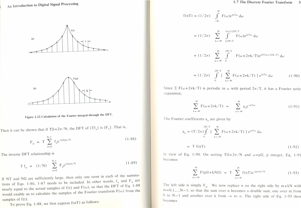
The proof of above equation requires a bit of algebra, I scanned 2 pages from a book I have on this (DSP by Liu and Peled) pages 38 and 39. Here it is (Click to enlarge).

And looking at equation 1-93 in the above.

2.2 on the second part

plot(f,2*abs(Y(1:NFFT/2+1)))
 

Why does it multiply by $2$?

First, they should not have multiplied by 2 the $Y(1)$ entry (i.e. the DC entry at frequency 0). The correct way would have been to do $2Y$, followed by $Y(1)=Y(1)/2$ to adjust the $Y$ at DC back to what it was before plotting it.

But the reason they multiplied $Y$ by $2$ is just normalization.

Matlab fft() returns Y(k) in the range $0$ to $f_s$ (with a $2\pi$ factor), and not from $0\cdots fs/2$.

So, the code was only using $Y(k)$ from $0\cdots \frac{f_s}{2}$, i.e. first half of the $Y(k)$.

Hence it was throwing away the part from $\frac{f_s}{2}\cdots f_s$.

Since $X(k)$ is symmetric, it was throwing away exactly half of the sequence $Y(k)$.

To keep the things equal (or to keep the energy the same, if you well, and I am being loose in the terms used here) as before throwing half of $Y$ away, we need to multiply by $2$ again to adjust it. (Similar to an area, which we cut in half, then to keep the area the same, we multiply the remaining area back by $2$).

The code above was plotting only half of $Y(k)$. You do not need to multiply by $2$ if you are plotting the whole $Y(k)$. Normally what is done is to use fftshift (which makes $Y(k)$ centered around 0 instead of how Matlab returns it)