Problem 5.24

Nasser Abbasi

Output

» nma_problem_5_24

nma_problem_5_24 - Program to compute the trajectories

of the Lorenz equations using the adaptive Runge-Kutta method.

then plot the power spectrum for z(t) solves problem 5.25

page 170

original program called lorenz, modified by Nasser Abbasi

Enter the initial position [x y z]: [1 1 20]

Enter the parameter r: 28

Enter number of steps: 1024

Finished 50 steps out of 1024

Finished 100 steps out of 1024

Finished 150 steps out of 1024

Finished 200 steps out of 1024

Finished 250 steps out of 1024

Finished 300 steps out of 1024

Finished 350 steps out of 1024

Finished 400 steps out of 1024

Finished 450 steps out of 1024

Finished 500 steps out of 1024

Finished 550 steps out of 1024

Finished 600 steps out of 1024

Finished 650 steps out of 1024

Finished 700 steps out of 1024

Finished 750 steps out of 1024

Finished 800 steps out of 1024

Finished 850 steps out of 1024

Finished 900 steps out of 1024

Finished 950 steps out of 1024

Finished 1000 steps out of 1024

»

source code

% nma_problem_5_24 - Program to compute the trajectories

% of the Lorenz equations using the adaptive Runge-Kutta method.

% then plot the power spectrum for z(t) solves problem 5.25

% page 170

% original program called lorenz, modified by Nasser Abbasi

clear; help nma_problem_5_24;

%* Set initial state x,y,z and parameters r,sigma,b

state = input('Enter the initial position [x y z]: ');

r = input('Enter the parameter r: ');

sigma = 10.; % Parameter sigma

b = 8./3.; % Parameter b

param = [r sigma b]; % Vector of parameters passed to rka

tau = 0.05; % timestep

%* Loop over the desired number of steps

time = 0;

nstep = input('Enter number of steps: ');

for istep=1:nstep

z_timeSeries(istep) = state(3); % save for power spectrum

%* Record values for plotting

x = state(1);

y = state(2);

z = state(3);

tplot(istep) = time;

tauplot(istep) = tau;

xplot(istep) = x;

yplot(istep) = y;

zplot(istep) = z;

if( rem(istep,50) < 1 )

fprintf('Finished %g steps out of %g\n',istep,nstep);

end

%* Find new state using adaptive Runge-Kutta

% [state, time, tau] = rka(state,time,tau,err,'lorzrk',param);

state = rk4(state,time,tau,'lorzrk',param);

time = time + tau;

end

%* Graph the time series z(t)

figure(1); clf; % Clear figure 1 window and bring forward

plot(tplot,zplot,'-')

xlabel('Time'); ylabel('z(t)')

title('Lorenz model z(t) time series')

pause(1) % Pause 1 second

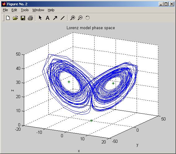
%* Graph the x,y,z phase space trajectory

figure(2); clf; % Clear figure 2 window and bring forward

% Mark the location of the three steady states

x_ss(1) = 0; y_ss(1) = 0; z_ss(1) = 0;

x_ss(2) = sqrt(b*(r-1)); y_ss(2) = x_ss(2); z_ss(2) = r-1;

x_ss(3) = -sqrt(b*(r-1)); y_ss(3) = x_ss(3); z_ss(3) = r-1;

plot3(xplot,yplot,zplot,'-',x_ss,y_ss,z_ss,'*')

view([30 20]); % Rotate to get a better view

grid; % Add a grid to aid perspective

xlabel('x'); ylabel('y'); zlabel('z');

title('Lorenz model phase space');

%

% power spectrum

%

f(1:nstep) = (0:(nstep-1))/(tau*nstep); % Frequency

z_fft = fft(z_timeSeries); % Fourier transform of z displacement

z_spect = abs(z_fft).^2; % Power spectrum of z displacement

%* Apply the Hanning window to the time series and calculate

% the resulting power spectrum

window = 0.5*(1-cos(2*pi*((1:nstep)-1)/nstep)); % Hanning window

z_w = z_timeSeries' .* window'; % Windowed time series

zw_fft = fft(z_w); % Fourier transf. (windowed data)

z_spectw = abs(zw_fft).^2; % Power spectrum (windowed data)

%* Graph the power spectra for original and windowed data

figure;

semilogy(f(1:(nstep/2)),z_spect(1:(nstep/2)),'b-',...

f(1:(nstep/2)),z_spectw(1:(nstep/2)),'r-');

title('Power spectrum for z(t) displacment (dashed is windowed data)');

xlabel('Frequency'); ylabel('Power');

legend('non-window data','window data');