Problem 9.12

Conclusion

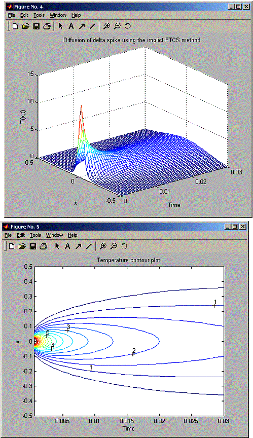
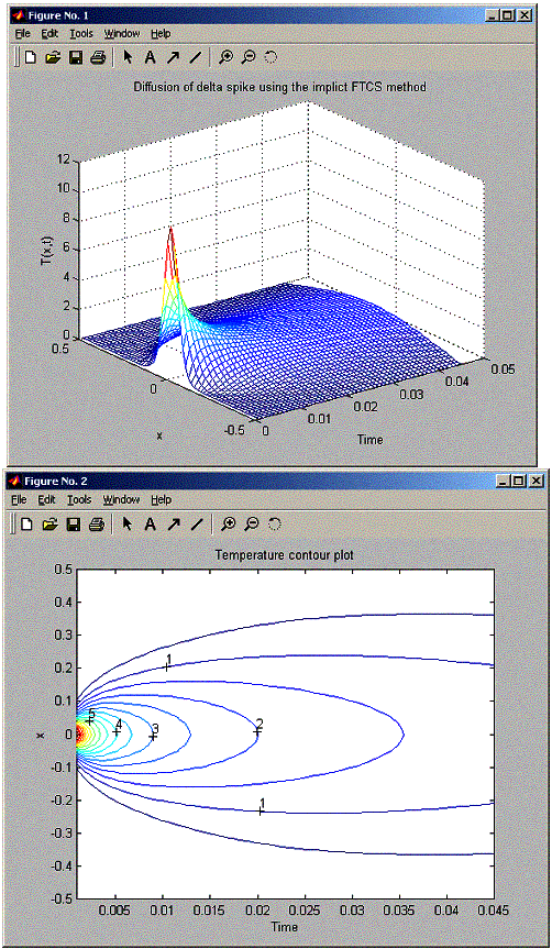
When running the implicit FTCS method and comparing to fig 6.7 and 6.8, found that when tau smaller than tsigma, the method is stable as with explicit FTCS fig 6.7. But when tau > tsigma, the explicit FTCS method (fig 6.8) showed it is unstable, however the implicit method showed that it is still stable even though tau > tsigma as can be seen by the plot below. So implicit FTCS is always stable.

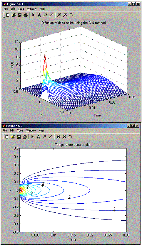
When running C-N method, it was also stable when tau> tsigma. The plots show C-N is similar to implicit FTCS method.

part a

OUTPUT

» nma_problem_9_12

function to solve problem 9.12

Nasser Abbasi

Enter N, number of grid points (suggest 61):61

Enter tau, the time step (suggest 1e-4 or 1.5e-4)1e-4

Enter nstep, the number of steps to run (suggest 300):300

Enter method 1=implicit FTCS, 2=Crank-Niclson:1

»

» nma_problem_9_12

function to solve problem 9.12

Nasser Abbasi

Enter N, number of grid points (suggest 61):61

Enter tau, the time step (suggest 1e-4 or 1.5e-4)1.5e-4

Enter nstep, the number of steps to run (suggest 300):300

Enter method 1=implicit FTCS, 2=Crank-Niclson:1

»

part b

» nma_problem_9_12

function to solve problem 9.12

Nasser Abbasi

Enter N, number of grid points (suggest 61):61

Enter tau, the time step (suggest 1e-4 or 1.5e-4)1e-4

Enter nstep, the number of steps to run (suggest 300):300

Enter method 1=implicit FTCS, 2=Crank-Niclson:2

»

» nma_problem_9_12

function to solve problem 9.12

Nasser Abbasi

Enter N, number of grid points (suggest 61):61

Enter tau, the time step (suggest 1e-4 or 1.5e-4)1.5e-4

Enter nstep, the number of steps to run (suggest 300):300

Enter method 1=implicit FTCS, 2=Crank-Niclson:2

»

code:

function nma_problem_9_12()

%

%function to solve problem 9.12

%Nasser Abbasi

%

% This is the same as dftc except we use the implicit

% Crank-Nicolson or the implicit FTCS method for

% solving the diffusion problem

%

clear all; help nma_problem_9_12;

L=1;

kappa=1; % diffusion coeff.

N=input('Enter N, number of grid points (suggest 61):');

h=L/(N-1);

tau=input('Enter tau, the time step (suggest 1e-4 or 1.5e-4)');

tsigma=h^2/(2*kappa);

coeff1= tau/(2*tsigma); % for FTCS

coeff2= tau/(4*tsigma); % for C-N

nstep=input('Enter nstep, the number of steps to run (suggest 300):');

method = input('Enter method 1=implicit FTCS, 2=Crank-Niclson:');

% make the D matrix based on Boundary conditions of Derchlit

D=makeD(N);

tt=zeros(N,1);

tt(round(N/2))=1/h ; %initial cond is delta at center

xplot = (0:N-1)*h - L/2; % xscale

iplot = 1; %counter for plots

nplots =50; % number of snapshots

plot_step=nstep/nplots;

% calculate the B matrix and use it in the loop

I=eye(N);

if(method ==1) % implict FTCS

B= inv(I-(coeff1*D));

else

B= inv(I - (coeff2*D)) * (I + (coeff2*D));

end

for istep=1:nstep

tt= B*tt; % this is the implicit method

if(rem(istep,plot_step)<1)

ttplot(:,iplot)=tt(:);

tplot(iplot)=istep*tau;

iplot = iplot+1;

end

end

figure;

mesh(tplot,xplot,ttplot);

xlabel('Time');

ylabel('x');

zlabel('T(x,t)');

if(method ==1)

title('Diffusion of delta spike using the implict FTCS method');

else

title('Diffusion of delta spike using the C-N method');

end

pause(1);

figure;

contourLevels=0:0.5:10;

contourLabels=0:5;

cs=contour(tplot,xplot,ttplot,contourLevels);

clabel(cs,contourLabels);

xlabel('Time');

ylabel('x');

title('Temperature contour plot');

%%%%%%%%%%%%%%%%%%%%%%%%%

%

%

%%%%%%%%%%%%%%%%%%%%%%%%%

function D=makeD(N)

D=zeros(N);

for(i=2:N-1)

D(i,(i-1))= 1;

D(i,(i)) = -2;

D(i,(i+1))= 1;

end