Project one. Problem 2. Mathematics 502 Probability and Statistics
Nasser Abbasi, September 26,2007. California State University, Fullerton

Part 2 (a)
The mixed distribution is
![]() -∞≤x≤∞
-∞≤x≤∞
Where ![]() is the density function for normal distribution with σ=1,μ=0, and
is the density function for normal distribution with σ=1,μ=0, and ![]() is the density function for normal distribution with σ=1,μ=3
is the density function for normal distribution with σ=1,μ=3
We need to generate random numbers from the above density function.
The following is the idea of how to solve this problem. Let us consider the case for γ=75% .Generate a r.v. from a uniform distribution, which will be between [0,1]. Let this number be called ζ. If ζ<.76 then now we will generate a random number from the above ![]() normal distribution otherwise we will generate a random number from
normal distribution otherwise we will generate a random number from ![]() distribution. Hence this is the algorithm
distribution. Hence this is the algorithm
Algorithm
Input: γ,![]() ,n (where n is number of random number to generate for mixture f(x)
,n (where n is number of random number to generate for mixture f(x)
output: n random numbers that belong to mixture f(x)
seed the random number generator (010101)
Initialize array d of the size of the random numbers generated
For i in 1..n LOOP
ζ = generate a r.v. from U[0,1]
IF ζ<γ THEN
d[i]= generate a random number from ![]()
ELSE
d[i]= generate a random number from ![]()
ENDIF
END LOOP
output d which will now contain n random variables drawn from the above probability density function.
Function to implement the mixture random variable algorithm
In[190]:=
![]()
In[192]:=

Now generate 2 sets of numbers each 10000 long, one for γ = .75 and the second for γ = .25
In[193]:=

Part 2 (b)
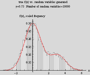
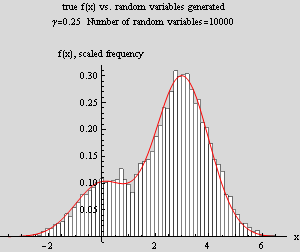
Generate 2 plots, one for γ = .75 and one for γ=.25 for number of random variables=10000 generated in part (a) overlaid by histogram.
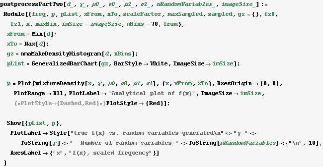
First define the mixture density function (the true density). Please see appendix for the code that overlays the histogram and the mixture function called postprocessPartTwo[]. Moved below to the appendix to reduce code clutter in the main report.
In[197]:=
![]()
Now call the above on the 2 sets of 10000 numbers generated in part (a) and display the result
This function makes a histogram which is scaled to be used to overlay density plots, or other functions.
Input: originalData: this is an array of numbers which represents the data to bin
nBins: number of bins
output: the histogram itself but scaled such that area is ONE
In[198]:=

In[200]:=
In[201]:=

Out[203]=
 |
 |
Comment and analysis on result of part 2 (b) plots
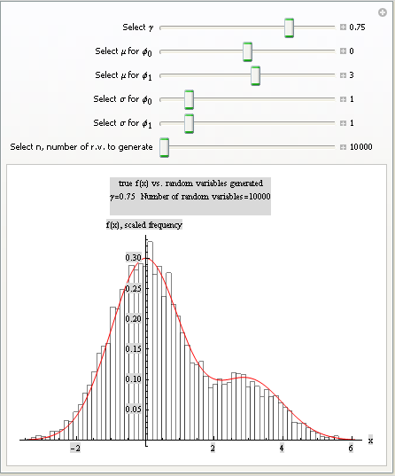
In the left plot, γ=.75, hence 75% of the mixture comes from ![]() which has a mean of 0, hence we would expect that at zero the bulk of the concentration, which what the plots shows to be the case (since both concentration have the same variance). Hence there should be more random numbers generated from this mixture around x=0 as well, and we see from the histogram that this is the case.
which has a mean of 0, hence we would expect that at zero the bulk of the concentration, which what the plots shows to be the case (since both concentration have the same variance). Hence there should be more random numbers generated from this mixture around x=0 as well, and we see from the histogram that this is the case.
In the right plot, now γ=.25, hence 75% of the concentration will come the ![]() distribution which has mean of 3. Hence again, we see that more random numbers are generated around 3 than anywhere else. These plots also show that the random numbers generated will have a probability density which will converge to the f(x) given as more and more random variables are generated.
distribution which has mean of 3. Hence again, we see that more random numbers are generated around 3 than anywhere else. These plots also show that the random numbers generated will have a probability density which will converge to the f(x) given as more and more random variables are generated.
Simulation program for problem 2
GUI to simulate part 2(b) of the project
In[204]:=

Out[204]=
In[205]:=
![]()
| Created by Wolfram Mathematica 6.0 for Students - Personal Use Only (25 September 2007) |