1.: up
2.: This page in PDF

(a)Problem review:

$T1$ is a random variable and $T2$ is a random variable, where $T1 ˜αe−αt1$ and $T2 ˜βe−βt2.$

$α$ and $β$ can be thought of as the failure rate for each respective component. $Ti$ is the lifetime of component $i$ . Hence $P (T1 = t1)$ means to ask for the probability of the ﬁrst component to have a lifetime of $t1$ given that the failure rate of this kind of components is $α.$

solution:

Now we know that

∫ ∫ P (T1 > T2) = fT1,T2 (t1,t2)dt2dt1

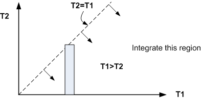
Looking at the following diagram to help determine the region to integrate:

Hence

∫ ∫ t1=∞ t2=t1 P (T1 > T2) = fT1,T2 (t1,t2)dt2 dt1 t1=0 t2=0

But since $T1 ⊥ T2,$ then the joint density is the product of the marginal densities.

Hence

Therefore

We take $α, β ≥ 0$ since we expect the lifetime to go to zero eventually. Also this is a requirement for the integrals to not diverge.

Hence the above becomes

Hence

|----------------------| | β | P (T1 > T2 ) = --------| ---------------(α-+-β)--

(b)

Hence

( ) ( ) fW (w ) = fT2 w- × d-- w- 2 dw 2

Hence

|--------------(---)-| | 1- w- | -fW-(w)-=-2-fT2--2---|

(c)Need to ﬁnd $P (T1 > 2T2 )$ which is the same as $P (T1 > W )$ , hence this is the same as part(a) but replace $T2$ by $W$ as show in the following diagram

Hence

Then

|------------------------| | β | |P (T1 > W ) = --------- | ---------------(2α-+-β-)-

Problem review: Poisson probability density is a discrete probability function (We normally call it the probability mass function $pmf$ ). This means the random variable is a discrete random variable.

The random variable $X$ in this case is the number of success in $n$ trials where the probability of success in each one trial is $p$ and the trials are independent from each others. The diﬀerence between Poisson and Binomial is that in Poisson we are looking at the problem as $n$ becomes very large and $p$ becomes very small in such a way that the product $np$ goes to a ﬁxed value which is called $λ$ , the Poisson parameter. 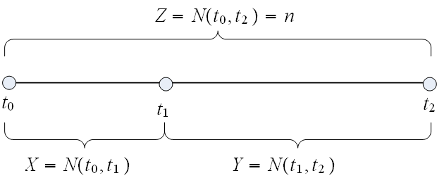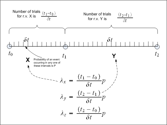And then we write $λk −λ P (X = k) = -k!e$ where $k = 0,1,2,⋅⋅⋅$ The following diagram illustrates this problem, showing the three r.v. we need to analyze and the time line.

But what is "trials" in this problem? If we divide the time line itself into very small time intervals $δt$ then the number of time intervals is the number of trials, and we assume that at most one event will occur in this time interval (since it is too small). The probability $p$ of event occurring in this $δt$ is the same in the interval $[t0,t1]$ and in the interval $[t1,t2]$ . Now let us ﬁnd $λ$ for $X$ and $Y$ and $Z$ based on this. Since $λ = np$ where $n$ is the number of trials, then for $X$ we have $λx = nxp = (t1−δtt0)p$ where we divided the time interval by the time width $δt$ to obtain the number of time slots for $X$ . We do the same for $Y$ and obtain that $(t2−t1)- λy = δt p$

Similarly, $(t− t) (t− t)+(t −t) (t −t) (t− t) λZ = --2δt0-p = -2--1δt-1--0p = -2δt1-p + -1δt0-P$ , hence $λz = λx + λy$

Let us refer to the random variable $N (t1,t2)$ as $Y$ and the r.v. $N (t0,t1)$ as $X$ and the r.v. $N (t0,t2)$ as $Z$

The problem is then asking to ﬁnd $P (X = x |Z = n)$ and to identify $pmf (X |Z )$

To help in the solution, we ﬁrst draw a diagram to make it more clear.

We take $λ$ to the same for the $3$ random variables $X, Y,Z$ .

P (X = x,Z = n) P (X = x|Z = n) = ------------------ P (Z = n)

But $Z = n$ is the same as $X + Y = n$ hence

Now r.v. $X$ $⊥ Y$ , since the number of events in $[t0, t1]$ is independent from the number of events that could occur in $[t1,t2]$ .

Given this, we can now write the joint probability of $X, Y$ as the product of the marginal probabilities. Hence the numerator in the above can be rewritten and we obtain

P (X = x|Z = n ) = P-(X--=-x)P--(Y--=-n-−-x-) P (Z = n)

(1)

Now since each of the above is a Poisson process, then

Hence (1) becomes

( x ) ( n− x ) P (X = x|Z = n) = (λx)-e−λx (λy-)---e− λy ---1n----- x! (n − x)! (λz)-e−λz n!

(2)

Hence

λ P (X = x|Z = n) = ----n!-----((λ )xe−λx) ((λ )n−xe −λy)-e-z-- x!(n − x )! x y (λz)n

But we found that $λ = λ + λ z x y$ , hence the exponential term above vanish and we get

Let $k = --λx- λx+λy$ , then $1 − k = 1 − --λx- = λx+λy−λx = --λy- λx+ λy λx+λy λx+λy$ hence the last line above can be written as

But this is a Binomial with parameters $n,k$ , hence

|----------------------------(----------)--| P (X = x |Z = n) ˜Binomial n, --λx---- | | λx + λy | --------------------------------------------

part (a)

Let $𝜃,$ the probability of getting heads, be the speciﬁc value that the random number $Θ$ can take.

Let $g(𝜃)$ be the probability density of $Θ$ , which we are told to be $U [0,1]$ , and let $pmf (x) X$ be the probability mass function of the random variable $X$ where $X$ is the number of times until a head ﬁrst comes up. $X$ is then a geometric random variable with parameter $𝜃$ , hence

N −1 pmfX (N ) = P (X = N ) = (1 − 𝜃) 𝜃 N = 1,2,3,⋅⋅⋅

The posterior density of $Θ$ given N is then

|-----------------------------------------------| | ---pmfX--(N-|Θ--=-𝜃)g-(𝜃)---| |h(Θ = 𝜃|X = N ) = ∫1 | ----------------------0-pmfX--(N-|Θ--=-𝜃)-g(𝜃)d𝜃--

But

pmfX (N |Θ = 𝜃) = (1 − 𝜃)N−1 𝜃

and $g(𝜃) = 1$ since $Θ ˜U [0,1]$

Hence

h (Θ = 𝜃 |X = N ) = ∫--(1-−-𝜃)N-−1𝜃--- 01(1 − 𝜃)N− 1𝜃 d𝜃

(1)

But $Θ$ is a random continuous variable from $[0,1]$ , so how to evaluate the above? I can evaluate the above for diﬀerent values of $Θ$ on the real line from $[0,1]$ , and the more values I take between $0,1$ the more accurate $h (Θ = 𝜃 |X = N )$ will become.

Part(b)

First let me evaluate eq (1) for $N = 1,N = 2,N = 6$

For $N = 1$

|--| h (Θ = 𝜃|X = 1) = ∫-𝜃----= [-𝜃]--= 2 𝜃| 1𝜃 d𝜃 𝜃2 1 ---- 0 2 0

For $N = 2$

For $N = 6$

(1 − 𝜃)6−1𝜃 (1 − 𝜃)5 𝜃 h(Θ = 𝜃|X = 6) = ∫-1-------6−-1-----= ∫1-------5----- 0 (1 − 𝜃) 𝜃 d𝜃 0 (1 − 𝜃) 𝜃 d𝜃

We can use integration by parts for the denominator, where $u = 𝜃,dv = (1 − 𝜃)5$ , when we do this we obtain

|------------| h (Θ = 𝜃 |X = 6) = |42 (1 − 𝜃)5 𝜃| --------------

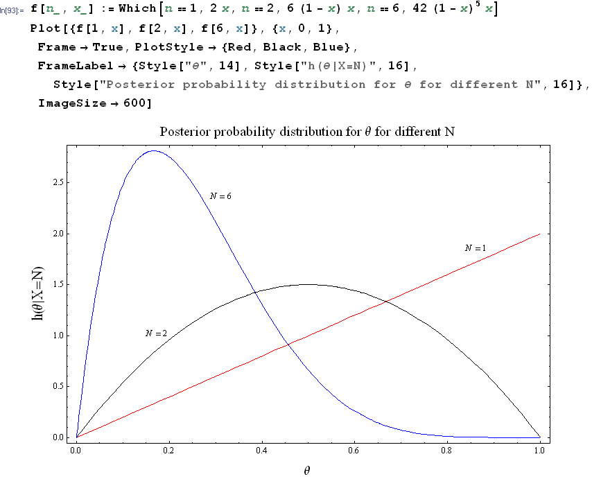
Now we plot the above 3 cases on the same plot:

What the above plot is saying is the following:

If it takes 'longer' to see a head comes up ( $N = 6$ ), then the coin is taken as biased towards a tail, and the probability of getting a head becomes smaller, this is why we see that the most likely probability in this case to be around $0.15$ (looking at the N=6 curve). We say that based on the observation of $N = 6$ , then the coin has a higher probability of having its probability of getting a head to be about $0.15$ than any other value. (The area around $𝜃 = 1.5$ is larger than any other area for the same $δ𝜃$ )

Now, when $N = 2$ , i.e. we ﬂipped the coin 2 times, and got a head on the second time, then we see from the $N = 2$ curve that the coin has a most likelihood of having a probability of getting a head to be 0.5 $.$

This is what we would expect, since in an unbiased coin, the probability of getting a head is $12$ , and hence with a fair coin, we expect to see a head half of the times it is ﬂipped, and since we ﬂipped 2 times, and saw a head the second time, this posterior probability has its most likely value to be around .5 as well.

When $N = 1$ , this says that we got a head in the ﬁrst time we ﬂipped the coin. We see that the posterior probability of getting a head now has it maximum around 1. This means the posterior probability is saying this coin is biased towards a head.

The above is a method to estimate the probability distribution of the probability itself of getting a head based on the observed events and based on the prior known probability of getting a head. Hence the events observed allow us to estimate the probability of getting a head. Hence the posterior probability is conditioned on each event as in this problem.