Computing assignment 3 Math 504. Spring 2008. CSUF craps and inventory problem
by Nasser Abbasi
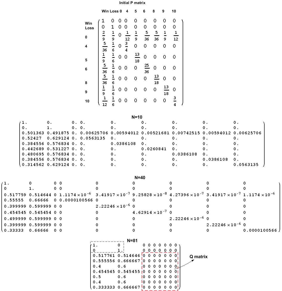
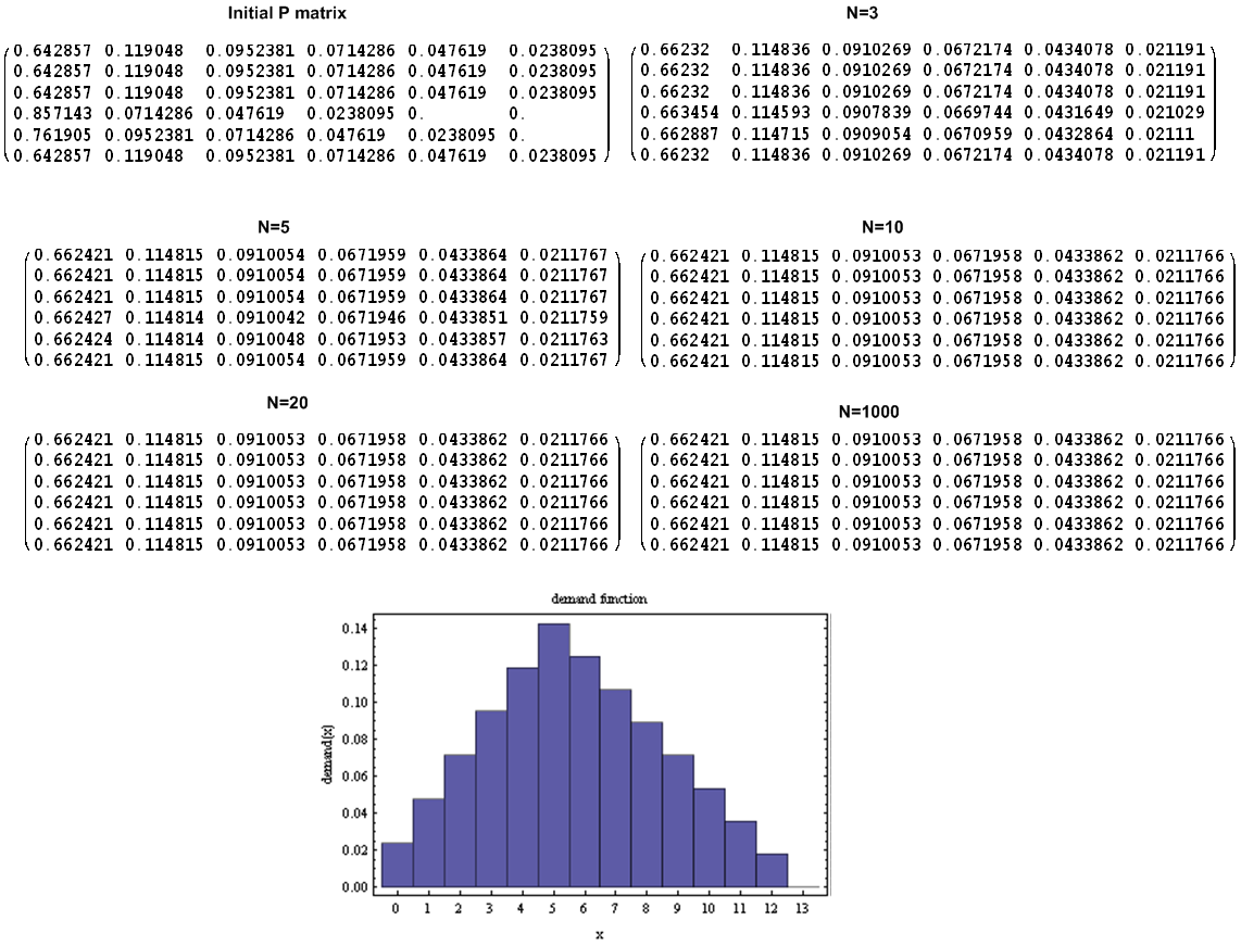
The state probability transition matrix was entered and then raised to higher powers. This is the numerical result
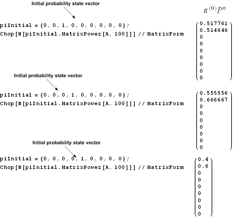
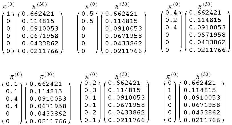
To answer part (b) below, we need to run the system from different initial
state vector (i.e. different
 )
and observe if the system probability state vector after a long time (i.e.
)
and observe if the system probability state vector after a long time (i.e.
 )
will depend on the initial state vector or not. Here is the result for 3
different initial state vectors. In diagram below we show the
)
will depend on the initial state vector or not. Here is the result for 3
different initial state vectors. In diagram below we show the
 and to its right
 .
.

 converges as
 .
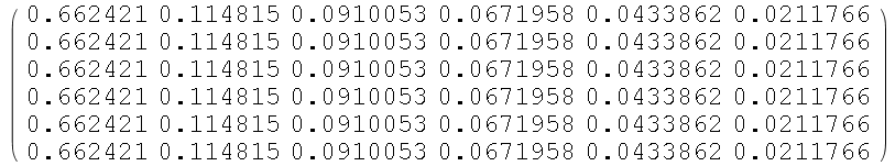
This is seen by looking at the above sequence of the
.
This is seen by looking at the above sequence of the
 matrix where we see that the matrix
 converges to the following limiting matrix at around

We can say the following about the limiting matrix: As
 the matrix
 converges to a fixed value shown above. The entries
 where
where
 is a transient state goes to zero as
 gets large.
From the above numerical result, we see that depending on the initial system
probability state vector
 we obtain a different system probability state vector
 as
as
 gets very large. This is because some states are transient (states
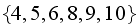 ).
In the inventory problem below, we see that we obtained a different result for
this part since the inventory problem has no transient states.
).
In the inventory problem below, we see that we obtained a different result for
this part since the inventory problem has no transient states.
Let
 be the set of all the possible states the system can be in. Hence from
definition, we
write
be the set of all the possible states the system can be in. Hence from
definition, we
write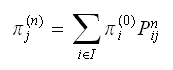
Where
 means the probability that the system will be in state
 after
after
 steps and
 is the
 steps transition probability. Now take the limit of the above as
 we
have
we
have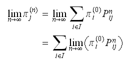 Assume there are
 states, we can
expand
states, we can
expand
But from part(a) we observed that in the limit, entries of each columns are
not equal. Hence
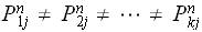 this means the above sum will produce a different value depending on the
initial state probability vector
this means the above sum will produce a different value depending on the
initial state probability vector
 .
(Compare this to the inventory problem below, where each entry in a column is
the same, and we could factor it out of the sum and we reached a different
conclusion than here).
.
(Compare this to the inventory problem below, where each entry in a column is
the same, and we could factor it out of the sum and we reached a different
conclusion than here).
Hence we showed depending on the initial
 then
then
 goes to different value as confirmed by the numerical result shown above in
part(a). Hence part(a) results could be used to deduce part(b) conclusion.
goes to different value as confirmed by the numerical result shown above in
part(a). Hence part(a) results could be used to deduce part(b) conclusion.
An inventory program was written in Mathematica (please see appendix for full
source code) which generated the
 matrix for an increasing values of
 .
The specification of the inventory model is described in the question shown
above. The value
.
The specification of the inventory model is described in the question shown
above. The value


The following are few results of the
 matrix for an increasing values of
 and the histogram of the demand distribution used.
To answer part (b) below, we need to run the system from different initial
state vector (i.e. different
 )
and observe if the system probability state after a long time (i.e.
)
and observe if the system probability state after a long time (i.e.
 )
will depend on the initial state vector or not. Since we know
that
)
will depend on the initial state vector or not. Since we know
that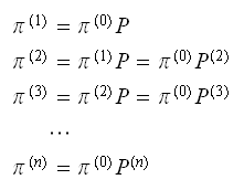 And since
 ,
then all what we have do is pick few
,
then all what we have do is pick few
 vectors, and post multiply them by
 for large
 and see if we obtain the same
 .
Below is the numerical result for this part showing the initial
.
Below is the numerical result for this part showing the initial
 and the final
 .
I used
.
I used
 in all cases as this showed it is large enough from the above numerical
results. Here are the results. Below we show result of 6 tests. In each one,
in all cases as this showed it is large enough from the above numerical
results. Here are the results. Below we show result of 6 tests. In each one,
 is shown and to its right
 .
.

 converges as
 .
This is seen by looking at the above sequence of the
.
This is seen by looking at the above sequence of the
 matrix where we see that the matrix
 converges to the following limiting matrix at around

We can say the following about the limiting matrix: As
 the matrix
 converges to a fixed value shown above. Each column has the same entries in
its rows. In addition, all entries are non-zero. This implies that the chain
contains no transient states. And since all the values on the converged
converges to a fixed value shown above. Each column has the same entries in
its rows. In addition, all entries are non-zero. This implies that the chain
contains no transient states. And since all the values on the converged
 matrix are positive, then we have only one closed set in the chain, which
contains all the states.
matrix are positive, then we have only one closed set in the chain, which
contains all the states.

 we obtain the same probability state vector
 when
when
 is large. So the final

In this part, we need to show given that
 converges to limiting fixed value, then the
 is the same for all states
 .
.
Let
 be the set of all the possible states the system can be in. Hence from
definition, we
write
be the set of all the possible states the system can be in. Hence from
definition, we
write Where
Where
 means the probability that the system will be in state
 after
after
 steps and
 is the
 steps transition probability. Now take the limit of the above as
 we
have
we
have Assume there are
 states, we can
expand
states, we can
expand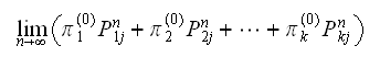
But from part(a) we observed that
 is a fixed value, which is the limit the transition matrix converged to. In
other words,
is a fixed value, which is the limit the transition matrix converged to. In
other words,
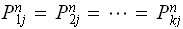 since all entries in the
 column are the same. Call this entry in
 column as
 say. So
 is a single number which represents the one step transition probability from
state
is a single number which represents the one step transition probability from
state
 to state
 when the system has run for a long time. So we write the above
as
when the system has run for a long time. So we write the above
as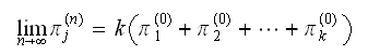 now,
now,
 is the sum of the probabilities of the system being in all its states at time
zero, which must be
is the sum of the probabilities of the system being in all its states at time
zero, which must be
 hence
hence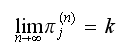 Hence we showed that regardless of the initial
 then
then
 goes to some fixed values. This shows that for any state
 the probability that the system will be in that state after a long time
converges to a fixed value regardless of the initial state if the system
transition matrix converges in the limit. Hence part(a) results could be used
to deduce part(b) conclusion.
the probability that the system will be in that state after a long time
converges to a fixed value regardless of the initial state if the system
transition matrix converges in the limit. Hence part(a) results could be used
to deduce part(b) conclusion.