HOME
HW 11 Mathematics 503, Mathematical Modeling,
CSUF , July 20, 2007
Nasser M. Abbasi
October 8, 2025
Contents
1 Problem 3 page 257 section 4.4 (Green Functions)
problem:
Consider boundary value problem \(u^{\prime \prime }-2xu^{\prime }=f\left ( x\right ) \),\(\ 0<x<1\), \(u\left ( 0\right ) =u^{\prime }\left ( 1\right ) =0\). Find Green function or explain where there isn’t
one.
answer:
We see that \(p\left ( x\right ) =-1\)
First, lets see if \(\lambda =0\) or not. Since if \(\lambda =0\) since by theorem 4.19 (page 248) Green function does not exist,
and I do not need to try to find it.
Let
\[ u^{\prime \prime }-2xu^{\prime }=\lambda u \]
If \(\lambda =0\,\ \) then solve the homogeneous equation \(u^{\prime \prime }-2xu^{\prime }=0\). Let \(y\left ( x\right ) =u^{\prime }\left ( x\right ) \), hence we obtain \(y^{\prime }-2xy=0\), by separation of variables, we
then have
\begin{align*} \frac {y^{\prime }}{y} & =2x\\ \frac {1}{y}dy & =2xdx\\ \int \frac {1}{y}dy & =2\int xdx \end{align*}
Hence
\[ \ln y=x^{2}+C \]
Which leads to \(y\left ( x\right ) =Ae^{x^{2}}\). But since \(y=u^{\prime }\), then \(\frac {du}{dx}=Ae^{x^{2}}\) or
\[ u\left ( x\right ) =A\int _{0}^{x}e^{t^{2}}dt+B \]
Therefore,
\[ \,u_{1}\left ( x\right ) =A\int _{0}^{x}e^{t^{2}}dt \]
and
\[ u_{2}\left ( x\right ) =B \]
At \(x=0\,\ \)we have \(u\left ( 0\right ) =0\), hence \(u\left ( 0\right ) =A\int _{0}^{0}e^{t^{2}}dt+B\) or \(0=B\) so now \(u\left ( x\right ) =A\int _{0}^{x}e^{t^{2}}dt\). Now lets see if this satisfies the second boundary condition \(u^{\prime }\left ( 1\right ) =0\). First
note that
\[ \frac {d}{dx}\left ( A\int _{0}^{x}e^{t^{2}}dt\right ) =Ae^{x^{2}}\]
hence \(\ \)at \(x=1\) we obtain \(0=A\exp \left ( 1\right ) \) which means \(A=0\), but this means trivial solution since both \(A,B\) are zero.
Hence \(\lambda \neq 0\) OK, so now I try to find Green function:
Now we need to find 2 independent solutions as combinations of \(A\int _{0}^{x}e^{t^{2}}dt\) and \(B\) such that each will satisfies
at least one of the boundary conditions.
We need \(u\left ( 0\right ) =0\), hence if we take
\[ u_{1}\left ( x\right ) =\int _{0}^{x}e^{t^{2}}dt \]
which will be zero at \(x=0\), and if we take
\[ u_{2}\left ( x\right ) =1 \]
then we see that \(u_{2}^{\prime }\left ( 1\right ) =0.\) Now find the
Wronskian
\[ W=\det \begin {bmatrix} u_{1} & u_{2}\\ u_{1}^{\prime } & u_{2}^{\prime }\end {bmatrix} =\det \begin {bmatrix} \int _{0}^{x}e^{t^{2}}dt & 1\\ e^{x^{2}} & 0 \end {bmatrix} =-e^{x^{2}}\]
Hence using equation 4.46 we obtain, noting that \(p=-1\)
\begin{align*} g\left ( x,\xi \right ) & =\left \{ \begin {array} [c]{cc}-\frac {u_{1}\left ( x\right ) u_{2}\left ( \xi \right ) }{p\ W\left ( \xi \right ) } & x<\xi \\ -\frac {u_{1}\left ( \xi \right ) u_{2}\left ( x\right ) }{p\ W\left ( \xi \right ) } & x>\xi \end {array} \right . =\left \{ \begin {array} [c]{cc}-\frac {u_{1}\left ( x\right ) u_{2}\left ( \xi \right ) }{\left ( -1\right ) \left ( \ -e^{\xi ^{2}}\right ) } & x<\xi \\ -\frac {u_{1}\left ( \xi \right ) u_{2}\left ( x\right ) }{\left ( -1\right ) \ \left ( -e^{\xi ^{2}}\right ) } & x>\xi \end {array} \right . \\ & =\left \{ \begin {array} [c]{cc}-e^{-\xi ^{2}}\int _{0}^{x}e^{t^{2}}dt & x<\xi \\ -e^{-\xi ^{2}}\int _{0}^{\xi }e^{t^{2}}dt & x>\xi \end {array} \right . \end{align*}
Hence
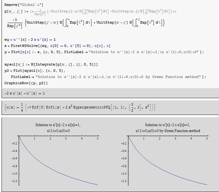
\[ \fbox {$g\left ( x,\xi \right ) =-e^{-\xi ^{2}}\left ( H\left ( \xi -x\right ) \int _{0}^{x}e^{t^{2}}dt+H\left ( x-\xi \right ) \int _{0}^{\xi }e^{t^{2}}dt\right ) $}\]
and
\[ u\left ( x\right ) =\int _{0}^{x}g\left ( x,\xi \right ) f\left ( \xi \right ) d\xi \]
I used the Green function I derived, and used it to plot the solution (for \(f\left ( x\right ) =1\)) and compare the plot
with the analytical solution.
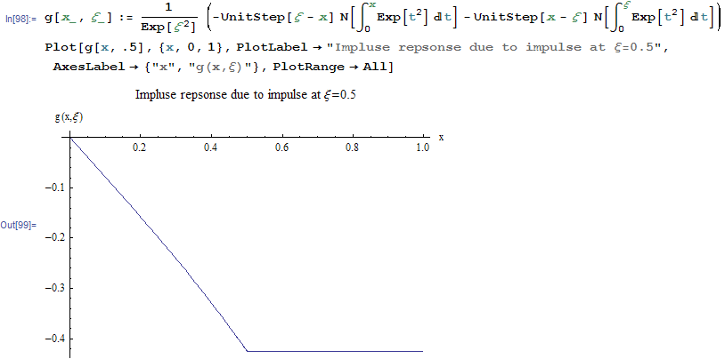
This is a plot of just the impulse response (green function) due to an impulse at \(x=0.5\)
This is another method to solving this problem by using properties of Green
function
From above we found \(u_{1}=\int _{0}^{x}e^{t^{2}}dt\), \(u_{2}=1\), but
\begin{align*} g\left ( x,\xi \right ) & =A\left ( \xi \right ) u_{1}\left ( x\right ) \ 0<x<\xi \\ & =A\left ( \xi \right ) \int _{0}^{x}e^{t^{2}}dt \end{align*}
and
\begin{align*} g\left ( x,\xi \right ) & =B\left ( \xi \right ) u_{2}\left ( x\right ) \\ & =B\left ( \xi \right ) \ \ \ \ \ \xi <x<1 \end{align*}
At \(x=\xi \), due to continuity, we require that
\begin{equation} A\left ( \xi \right ) \int _{0}^{\xi }e^{t^{2}}dt=B\left ( \xi \right ) \tag {1}\end{equation}
and to impose the discontinuity condition on the first derivative we have
\begin{align} g^{\prime }\left ( \xi ^{+},\xi \right ) -g^{\prime }\left ( \xi ^{-},\xi \right ) & =\frac {-1}{p\left ( \xi \right ) }\nonumber \\ 0-A\left ( \xi \right ) e^{\xi ^{2}} & =1\nonumber \\ A\left ( \xi \right ) & =\frac {-1}{e^{\xi ^{2}}} \tag {2}\end{align}
From (1) we then obtain that
\[ B\left ( \xi \right ) =\frac {-1}{e^{\xi ^{2}}}\int _{0}^{\xi }e^{t^{2}}dt \]
Hence
\begin{align*} g\left ( x,\xi \right ) & =A\left ( \xi \right ) u_{1}\left ( x\right ) \ \ \\ & =\frac {-1}{e^{\xi ^{2}}}\int _{0}^{x}e^{t^{2}}dt\ \ \ \ \ \ \ 0<x<\xi \end{align*}
and
\begin{align*} g\left ( x,\xi \right ) & =B\left ( \xi \right ) u_{2}\left ( x\right ) \\ & =\frac {-1}{e^{\xi ^{2}}}\int _{0}^{\xi }e^{t^{2}}dt\ \ \ \ \ \ \ \ \ \xi <x<1 \end{align*}
Hence
\[ \fbox {$g\left ( x,\xi \right ) =\frac {-1}{e^{\xi ^{2}}}\left ( H\left ( \xi -x\right ) \int _{0}^{x}e^{t^{2}}dt+H\left ( x-\xi \right ) \int _{0}^{\xi }e^{t^{2}}dt\ \right ) $}\]
Compare this solution to the one found above using the formula method we see they are the
same.
2 Problem 8, page 258 section 4.5
Problem:
Find the inverse of the differential operator \(Lu=-\left ( x^{2}u^{\prime }\right ) ^{\prime }\) on \(1<x<e\) subject to \(u\left ( 1\right ) =u\left ( e\right ) =0\)
solution:
This is SLP problem with \(p=x^{2},q=0\). First find if \(\lambda =0\) is possible eigenvalue.
\[ \lambda u=-\left ( x^{2}u^{\prime }\right ) ^{\prime }\]
Let \(\lambda =0\), hence we have \(-\left ( x^{2}u^{\prime }\right ) ^{\prime }=0\) or \(-\left ( 2xu^{\prime }+x^{2}u^{\prime \prime }\right ) =0\) or
\[ u^{\prime \prime }+\frac {2}{x}u^{\prime }=0 \]
Use separation of variables. First let \(y=u^{\prime }\), hence \(y^{\prime }+\frac {2}{x}y=0\) or \(\frac {1}{y}\frac {dy}{dx}=-\frac {2}{x}\) hence
\begin{align*} \int \frac {1}{y}dy & =-2\int \frac {1}{x}dx\\ \ln y & =-2\ln x+c\\ y & =Ae^{-2\ln x}\\ y & =A\frac {1}{x^{2}}\end{align*}
But \(y=u^{\prime }\), hence \(du=A\frac {1}{x^{2}}dx\) or \(u=A\int \frac {1}{x^{2}}dx\)
hence \(u=-A\frac {1}{x}+B\) or
\[ \fbox {$u\left ( x\right ) =\frac {A}{x}+B$}\]
where the minus sign is absorbed into \(A\). Hence we have 2 independent solutions \(\frac {A}{x}\) and \(B\), so
we need combination of these 2 solutions to satisfy the BV. At \(x=1\) we have \(u=0\), hence if we take \(u_{1}=\frac {1}{x}-1\) then it
will satisfy this condition. At \(x=e\) we need \(u=0\), hence take \(u_{2}=\frac {1}{x}-\exp \left ( -1\right ) \)
Then
\[ W=\det \begin {bmatrix} u_{1} & u_{2}\\ u_{1}^{\prime } & u_{2}^{\prime }\end {bmatrix} =\det \begin {bmatrix} \frac {1}{x}-1 & \frac {1}{x}-\exp \left ( -1\right ) \\ \frac {-1}{x^{2}} & \frac {-1}{x^{2}}\end {bmatrix} =-e^{x^{2}}\]
Hence
\[ W=\frac {1-e^{-1}}{x^{2}}\]
Then green function is
\begin{align*} g\left ( x,\xi \right ) & =\left \{ \begin {array} [c]{cc}-\frac {u_{1}\left ( x\right ) u_{2}\left ( \xi \right ) }{W\left ( \xi \right ) } & x<\xi \\ -\frac {u_{1}\left ( \xi \right ) u_{2}\left ( x\right ) }{W\left ( \xi \right ) } & x>\xi \end {array} \right . =\left \{ \begin {array} [c]{cc}-\frac {\left ( \frac {1}{x}-1\right ) \left ( \frac {1}{\xi }-e^{-1}\right ) }{\xi ^{2}\frac {1-e^{-1}}{\xi ^{2}}} & x<\xi \\ -\frac {\left ( \frac {1}{\xi }-1\right ) \left ( \frac {1}{x}-e^{-1}\right ) }{\xi ^{2}\frac {1-e^{-1}}{\xi ^{2}}} & x>\xi \end {array} \right . \\ & \left \{ \begin {array} [c]{cc}\left ( 1-\frac {1}{x}\right ) \frac {\left ( 1-\xi e^{-1}\right ) }{\xi \left ( e^{-1}-1\right ) } & x<\xi \\ \left ( \frac {1}{x}-e^{-1}\right ) \frac {\left ( 1-\xi \right ) }{\xi \left ( e^{-1}-1\right ) } & x>\xi \end {array} \right . \end{align*}
But the inverse \(L^{-1}\) is \({\displaystyle \int } g\left ( x,\xi \right ) f\left ( x\right ) dx\) where \(g\left ( x,\xi \right ) \) is the green function given aboive.
Another way to solve the problem:
From above we found \(u_{1}=\frac {1}{x}-1\), \(u_{2}=\frac {1}{x}-e^{-1}\), but
\begin{align*} g\left ( x,\xi \right ) & =A\left ( \xi \right ) u_{1}\left ( x\right ) \ \\ & =A\left ( \xi \right ) \left ( \frac {1}{x}-1\right ) \ \ \ \ \ 1<x<\xi \end{align*}
and
\begin{align*} g\left ( x,\xi \right ) & =B\left ( \xi \right ) u_{2}\left ( x\right ) \\ & =B\left ( \xi \right ) \ \left ( \frac {1}{x}-e^{-1}\right ) \ \ \ \ \ \xi <x<e \end{align*}
At \(x=\xi \), due to continuity, we require that
\begin{equation} A\left ( \xi \right ) \left ( \frac {1}{\xi }-1\right ) =B\left ( \xi \right ) \ \left ( \frac {1}{\xi }-e^{-1}\right ) \tag {1}\end{equation}
and to impose the discontinuity condition on the first derivative we have
\begin{align} g^{\prime }\left ( \xi ^{+},\xi \right ) -g^{\prime }\left ( \xi ^{-},\xi \right ) & =\frac {-1}{p\left ( \xi \right ) }\nonumber \\ B\left ( \xi \right ) \ \left ( \frac {-1}{\xi ^{2}}\right ) -A\left ( \xi \right ) \left ( \frac {-1}{\xi ^{2}}\right ) & =\frac {-1}{\xi ^{2}}\nonumber \\ B\left ( \xi \right ) \ -A\left ( \xi \right ) & =1 \tag {2}\end{align}
Solve (1) and (2) for \(B\left ( \xi \right ) ,A\left ( \xi \right ) \)
From (2) we have\(B\left ( \xi \right ) =1+A\left ( \xi \right ) \)\(,\)substitute into (1) we have \(A\left ( \xi \right ) \left ( \frac {1}{\xi }-1\right ) =\left ( 1+A\left ( \xi \right ) \right ) \ \left ( \frac {1}{\xi }-e^{-1}\right ) \) or
\begin{align*} \frac {A\left ( \xi \right ) }{\xi }-A\left ( \xi \right ) & =\ \frac {1}{\xi }-e^{-1}+\frac {A\left ( \xi \right ) }{\xi }-A\left ( \xi \right ) e^{-1}\\ -A\left ( \xi \right ) +A\left ( \xi \right ) e^{-1} & =\frac {1}{\xi }-e^{-1}\\ A\left ( \xi \right ) \left ( e^{-1}-1\right ) & =\frac {1}{\xi }-e^{-1}\\ A\left ( \xi \right ) & =\frac {1-\xi e^{-1}}{\xi \left ( e^{-1}-1\right ) }\end{align*}
Hence
\begin{align*} B\left ( \xi \right ) & =1+A\left ( \xi \right ) \\ & =1+\frac {1-\xi e^{-1}}{\xi \left ( e^{-1}-1\right ) }\\ & =\frac {1-\xi }{\xi \left ( e^{-1}-1\right ) }\end{align*}
Then
\begin{align*} g\left ( x,\xi \right ) & =A\left ( \xi \right ) u_{1}\left ( x\right ) \ \\ & =\left ( \frac {1-\xi e^{-1}}{\xi \left ( e^{-1}-1\right ) }\right ) \left ( \frac {1}{x}-1\right ) \ \ \ \ \ 1<x<\xi \end{align*}
\begin{align*} g\left ( x,\xi \right ) & =B\left ( \xi \right ) u_{2}\left ( x\right ) \\ & =\left ( \frac {1-\xi }{\xi \left ( e^{-1}-1\right ) }\right ) \left ( \frac {1}{x}-e^{-1}\right ) \ \ \ \ \ \ \ \ \xi <x<e \end{align*}
Hence
\[ \fbox {$g\left ( x,\xi \right ) =\frac {1}{e^{\xi ^{2}}}\left ( H\left ( \xi -x\right ) \left ( \frac {1-\xi e^{-1}}{\xi \left ( e^{-1}-1\right ) }\right ) \left ( \frac {1}{x}-1\right ) +H\left ( x-\xi \right ) \left ( \frac {1-\xi }{\xi \left ( e^{-1}-1\right ) }\right ) \left ( \frac {1}{x}-e^{-1}\right ) \ \right ) $}\]
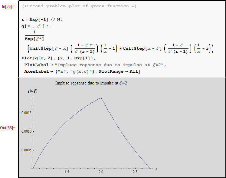
Which agree with the formula method.
This a plot of Green function for \(\xi =2\)