HOME

Contents

1 Problem 8 page 362 section 6.3

problem:

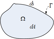
Consider the problem of minimizing the functional \(J\left ( u\right ) ={\displaystyle \int \limits _{\Omega }} L\left ( \mathbf {x},u,\nabla u\right ) d\mathbf {x}\) over all \(u\in C^{2}\left ( \Omega \right ) \) with \(u\left ( \mathbf {x}\right ) =f\left ( \mathbf {x}\right ) \) at boundary \(\Gamma \) where \(f\) is a given function. \(\Omega \) is bounded and well behaved in \(\mathbb {R} ^{2}.\)

(a) Show that the first variation is (Where \(L\) below is meant to be \(L\left ( \mathbf {x},u,\nabla u\right ) \) ) where \(\mathbf {x}\) is the vector \(\begin {bmatrix} x_{1}\\ x_{2}\end {bmatrix} \)

Where \(L_{\nabla u}\) is the vector \(\begin {bmatrix} L_{\left ( \frac {\partial u}{\partial x_{1}}\right ) }\\ L_{\left ( \frac {\partial u}{\partial x_{2}}\right ) }\end {bmatrix} =\begin {bmatrix} \frac {\partial L}{\partial \left ( \frac {\partial u}{\partial x_{1}}\right ) }\\ \frac {\partial L}{\partial \left ( \frac {\partial u}{\partial x_{2}}\right ) }\end {bmatrix} \) and \(\mathbf {h}\in C^{2}\left ( \Omega \right ) \) with \(h\left ( \mathbf {x}\right ) =\mathbf {0}\) at the boundary \(\Gamma \)

(b)Show that the necessary condition for \(u\) to minimize \(J\) is that \(u\) must satisfy the Euler equation \(L_{u}\mathbf {-\nabla \cdot }L_{\nabla u}=0\), \(\mathbf {x}\in \Omega \)

(c)If \(u\) is not fixed on the boundary \(\Gamma \) find the natural boundary conditions.

Answer

(a)

Hence

But \(\delta J\left ( u,\mathbf {h}\right ) =\lim _{t\rightarrow 0}\frac {dJ\left ( u+th\right ) }{dt}\), hence at \(t=0\) the above becomes

But \(\nabla u=\begin {bmatrix} \frac {\partial u}{\partial x_{1}}\\ \frac {\partial u}{\partial x_{2}}\end {bmatrix} \), hence \(\frac {\partial L}{\partial \left ( \nabla u\right ) }=\begin {bmatrix} \frac {\partial L}{\partial \left ( \frac {\partial u}{\partial x_{1}}\right ) }\\ \frac {\partial L}{\partial \left ( \frac {\partial u}{\partial x_{2}}\right ) }\end {bmatrix} \), and \(\nabla h=\begin {bmatrix} \frac {\partial h}{\partial x_{1}}\\ \frac {\partial h}{\partial x_{2}}\end {bmatrix} \), therefore

Hence (1) becomes

Now

Hence

Hence substitute the above in (2) for \(i=1,2\) we obtain

Now using Green theorem, where

Let \(Q\equiv L_{u_{x_{1}}}h,P\equiv -L_{u_{x_{2}}}h\), hence Green theorem becomes

Substitute the above into second term in (3) we obtain (noting that \(dA=dx_{1}dx_{2}\) since we are in \(\mathbb {R} ^{2}\))

But the second integral above can be rewritten as (by dividing and multiplying by \(ds\))

Hence (4) becomes

Now Tangent vector at the boundary at point \((x_{1},x_{2})\) is given by vector \(\left ( \frac {dx_{1}}{ds},\frac {dx_{2}}{ds}\right ) ^{T}\), hence the normal is \(\mathbf {n}=\left ( \frac {dx_{2}}{ds},-\frac {dx_{1}}{ds}\right ) ^{T}\) (since if we take dot product of these 2 vectors we get zero).  Now we can rewrite the integrand in the second integral in (5) in terms of this normal vector since

Substitute the above into the second term of (5) we obtain

Final note on the sign before the second integral above. The book shows it as \("-"\). I think this is because the normal should be pointing outside? Hence if we make out normal the negative of the normal used here (which I think points inwards), we obtain the result we are asked to show for part (a). (notice, the book has a mistake/typo, it says \(\int _{\Gamma }h\left ( L_{\nabla u}\cdot \mathbf {n}\right ) \ \ dA\) instead of \(\int _{\Gamma }h\left ( L_{\nabla u}\cdot \mathbf {n}\right ) \ \ ds\), i.e. the integration is over a line segment, not over a differential area (since obviously this is contour integration).

part (b)

Necessary condition for minimum is that \(\delta J\left ( u,\mathbf {h}\right ) =0\),. ie.

Now consider the second integral in the above. Since \(h=0\) on \(\Gamma \), hence we are left to show that

But \(h\) is arbitrary function, hence by lemma 3.13 again, we argue that for the above to be zero, then

Which is Euler-Lagrange equation.

Part (c)

Here we have free boundary conditions. Hence we can not take \(h=0\) everywhere on \(\Gamma \). Starting with the first variation

Since \(h\neq 0\) on \(\Gamma \,\ \)then by lemma 3.13 we can argue that \(L_{\nabla u}\cdot \mathbf {n=0}\) on \(\Gamma \)

Hence on \(\mathbb {R} ^{2}\), this means \(\begin {bmatrix} L_{u_{x_{1}}}\\ L_{u_{x_{2}}}\end {bmatrix} ^{T}\begin {bmatrix} \frac {dx_{2}}{ds}\\ -\frac {dx_{1}}{ds}\end {bmatrix} =0\), i.e.

Now we need to know the shape of the boundary to evaluate the above at each point. For example, for a circle, \(\mathbf {n}=\begin {bmatrix} x_{1}\\ x_{2}\end {bmatrix} \) and the above become

And the above equation needs to be satisfied at each point on the boundary after discretization.