To run the program, please copy the content of the floppy disk (which contains the required 2 matlab files, one is called nma_185_proj3.m, and the other is a utility support file called nma_inputNumeric.m) to your MATLAB work folder on your C: drive.
The MATLAB work folder will be located under the main MATLAB folder. The name of the MATLAB main folder depends on the version of MATLAB you have installed. For example, for MATLAB 6.5, it is called
Once the files are copied to the work folder below the above MATLAB main folder, then start matlab itself, and from the matlab console, type the command:
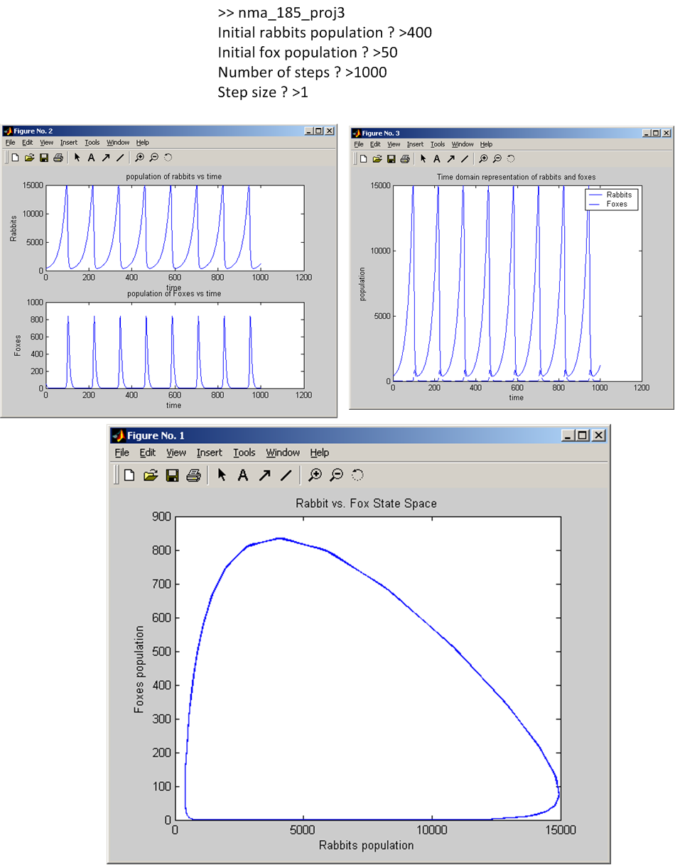
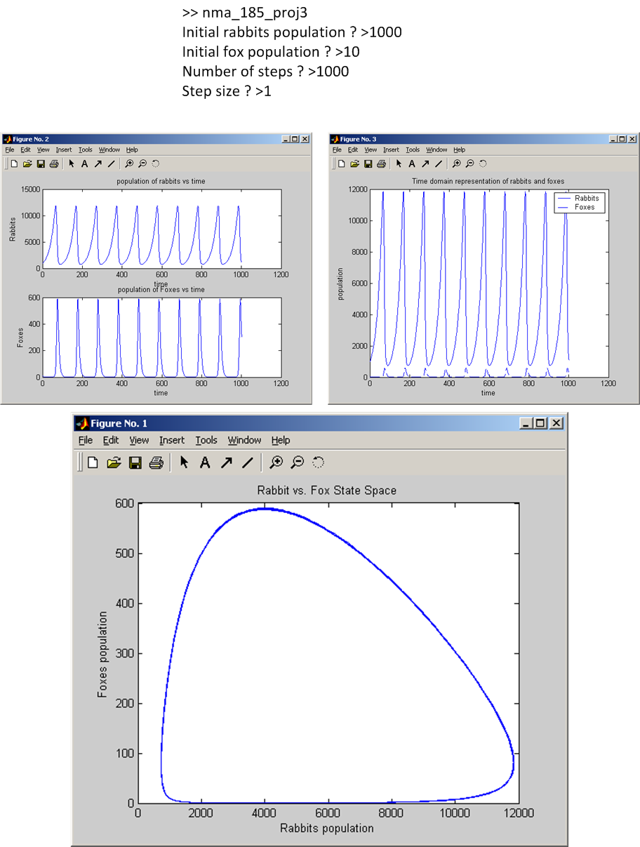
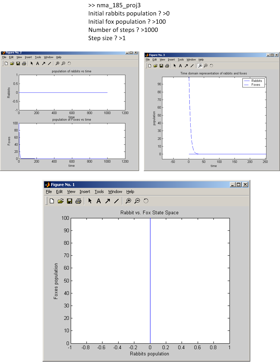
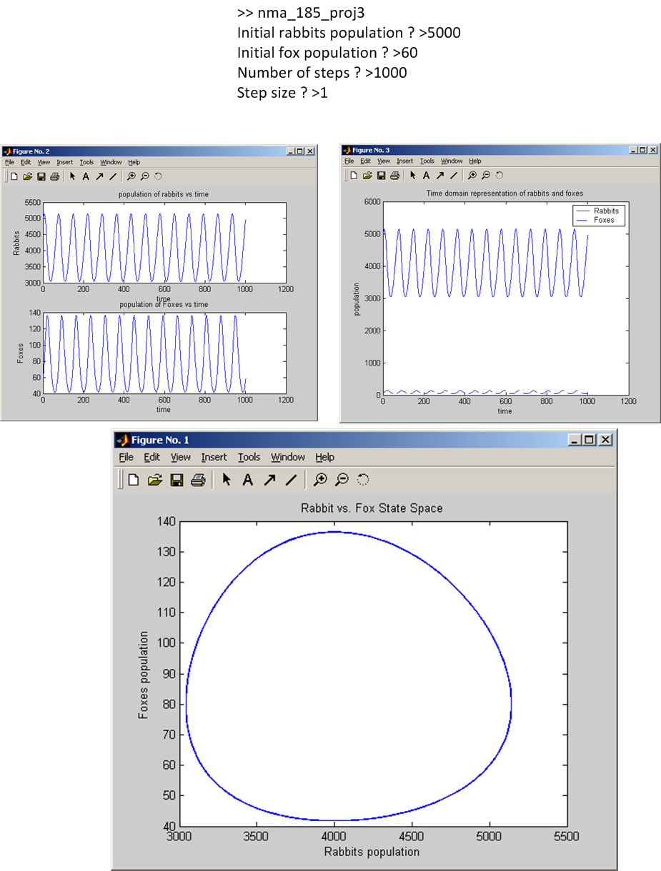
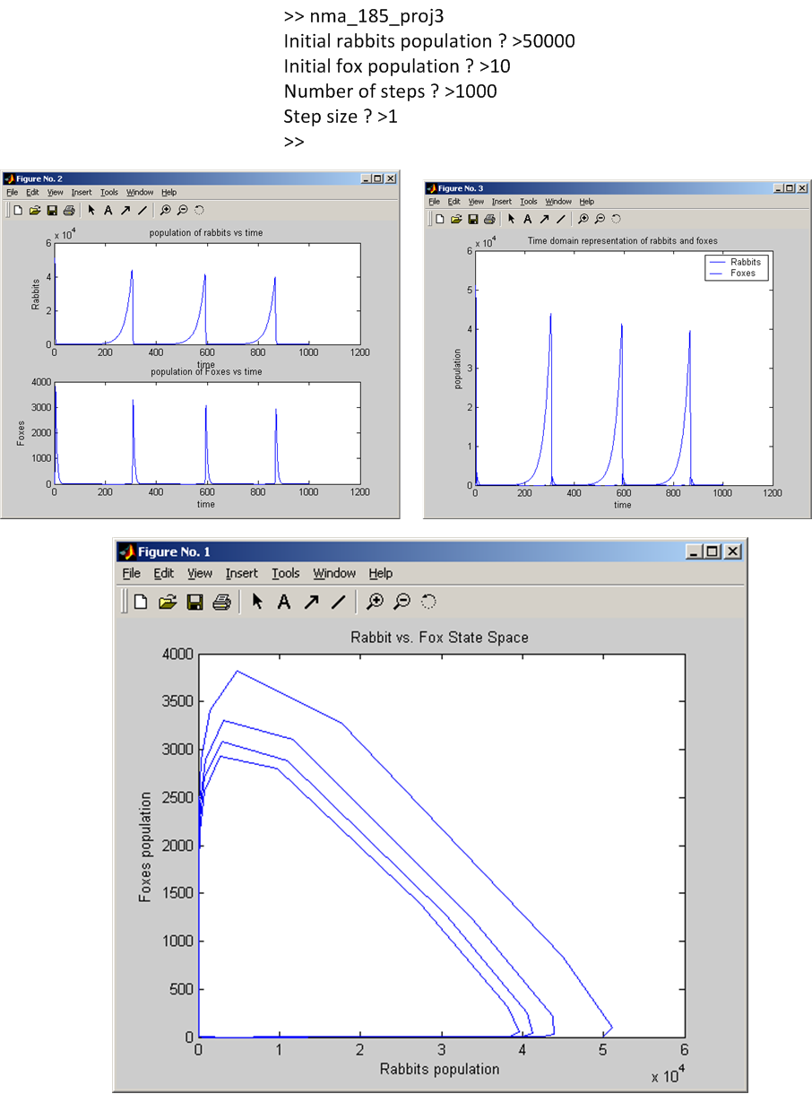
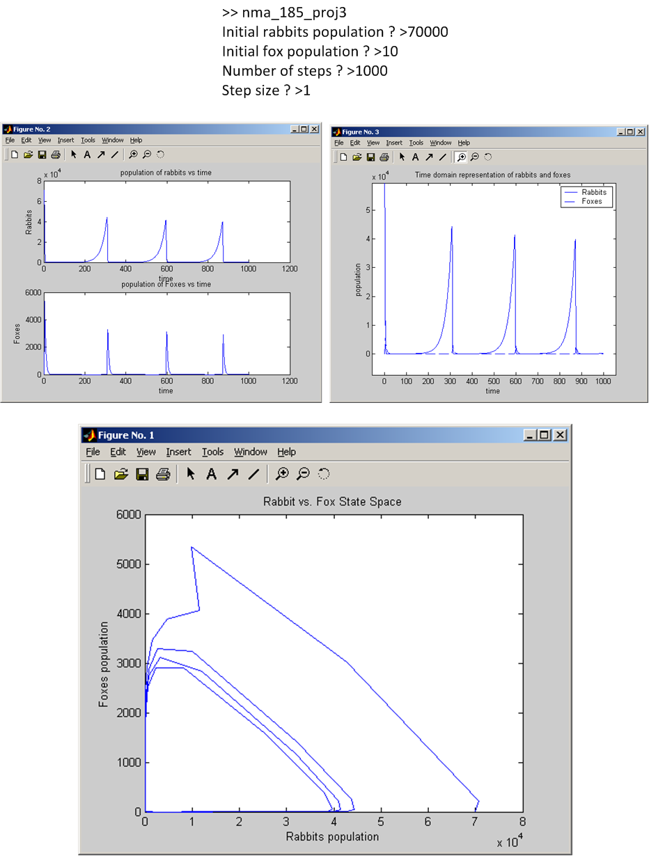
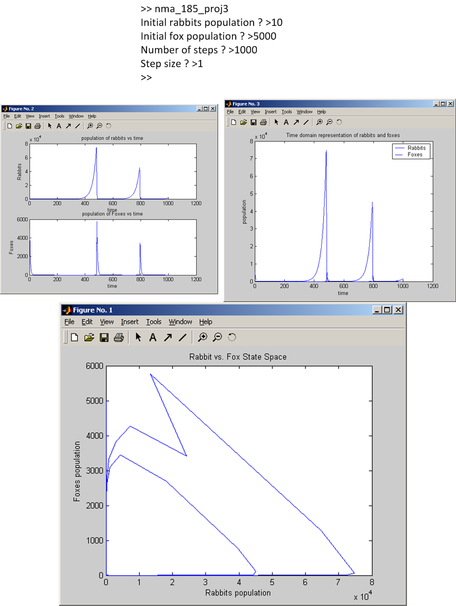
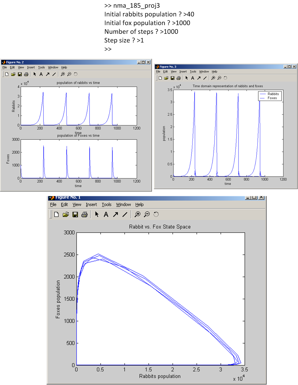
The program now will start and asks for input. This is an example of the required input from one test run:
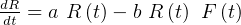
The program will then solve the problem and will display 3 different figure windows to show the results. It will display the state-space solution, the time-domain solution for each independent variable, both on the same plot and on separate plots. Please see test cases below for more examples.
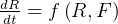
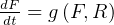
Let prey by rabbits (R), and predators be foxes (F). Model is

Where
 is natural growth of R in absence of F.
 is natural death rate of F in absence of its food R.
 is the death rate per encounter of R due to predation.
 is the efficiency of turning predated R into F.
Solve the couple ODE using Runge-Kutta 4th order classical method.
Use the following values for the above parameters:


Try different initial conditions for R and F population.
let 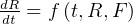
let 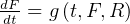
Since the rate of population is not explicitly given in terms of the independent variable  I could write the
above as
I could write the
above as
But for generality, I will keep the first form.
To solve using R-K 4th order method, then we write


Let  , the step size.
The only trick in these coupled ODE is the order in which we evaluate the K coefficients. This can be seen
when we write the K down. When writing the K coefficients down, use this notation  to mean the
  K
for rabbits. And
K
for rabbits. And  to mean the
  K for Foxes. This means the second subscript represents the
independent variable. This will reduce confusion and mistakes.
K for Foxes. This means the second subscript represents the
independent variable. This will reduce confusion and mistakes.
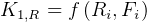


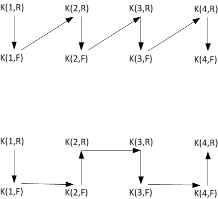
Hence, looking at the dependency of the  above, we see some possible sequential ordering in which to
evaluate those
above, we see some possible sequential ordering in which to
evaluate those  for each step. See diagram 1
I will pick the first ordering sequence above for the implementation.
The above gives all the setup I need to implement the algorithm. This is implemented in MATLAB function called nma_185_proj2.m. The function asks the user for the initial population of the F and R, and the number of time steps, and for the size of the time step and will display the solution obtained.
The file nma_185_proj3.m is moved to my main matlab functions page here