LAB #5 report. MAE 106. UCI. Winter 2005
Nasser Abbasi, LAB time: Thursday 2/10/2005 6 PM
a)
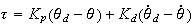
The output is
 and the input is

But

Take Laplace transform we get
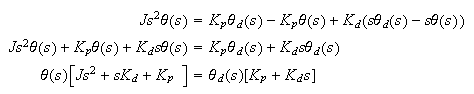
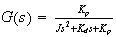
Hence the transfer function
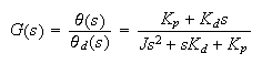
Compare this transfer function with
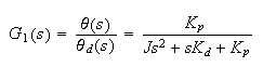 the
one we used in the Lab. We see that new
the
one we used in the Lab. We see that new
 has a zero at
 while
while
 has no zero. This controller will perform better as it tracks speed error as
well as position error. This will make it more sensitive to changes.
has no zero. This controller will perform better as it tracks speed error as
well as position error. This will make it more sensitive to changes.
 For
p1, we are asked to plot the predicted response of
For
p1, we are asked to plot the predicted response of
 for a step input for

Write the equation in standard form, we get
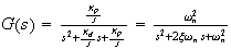
Hence
 and
and

Where
 and
and

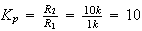
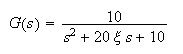
I will use
 hence
the transfer function becomes
hence
the transfer function becomes
The following are the plots generated by a small program
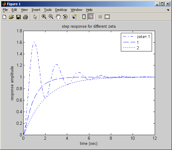
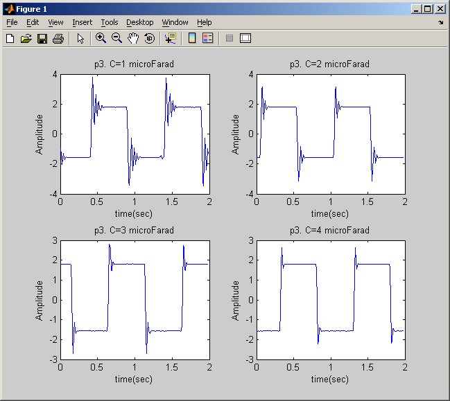
For p3, we are asked to show plots for step input response for
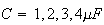 These are plots:
for
p4, we are asked to plot the step response with higher k on top of the step
response using original gain. this is the result
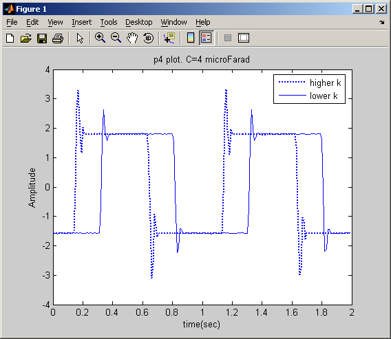
We see that with higher k, then the system responded more quickly.
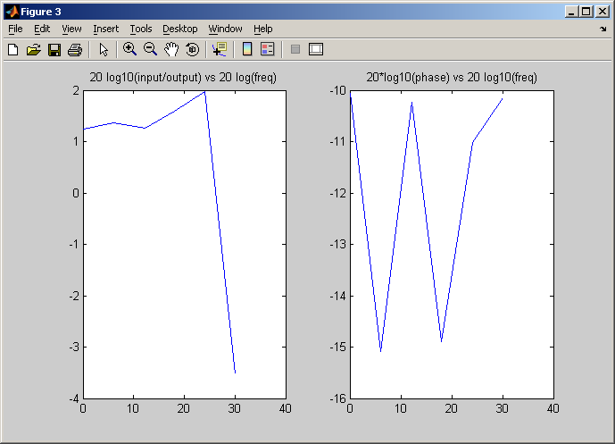
Here we are asked to plot the frequency response for the predicted response. p2:
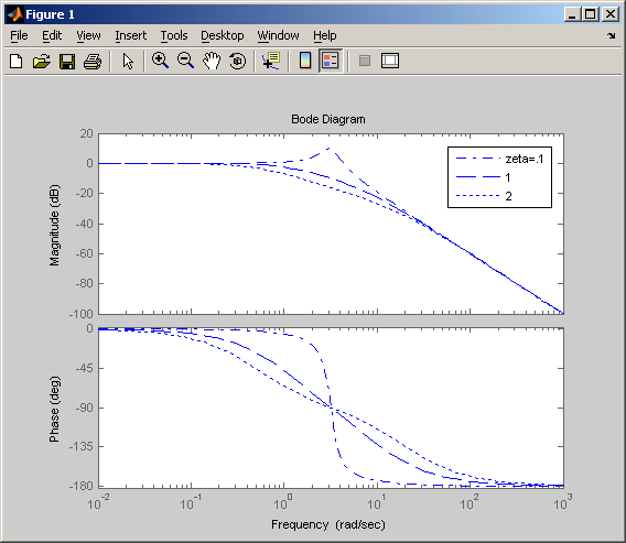
This is the result for p5