Image Restoration by Inverse Filtering in the Frequency Domain Using Gaussian and Ideal Low Pass Filters
By Nasser M. Abbasi
Introduction
This report was written during Fall 2004. EECS 207A. UCI.
This is an implementation of a standard algorithm for 2D gray image restoration which is based on a mathematical model of image degradation.
Image restoration attempts to recover, as much as possible, the original image from the degraded image, using knowledge of the process that caused the degradation itself.
The restoration algorithm used assumes we know the mathematical model of the degradation that we are trying to remove.
Degradation is caused by either blur or by noise. There are algorithms to do restoration in the frequency domain and those that do the restoration directly in the spatial domain.
There are algorithms that concentrate on reversing the effects of noise only, those that concentrate on removing the effects of blur, and those that attempt to remove the effect of both noise and blur.
This project is an implementation of an algorithm that works in the frequency domain which inverts the effect of blur only.
To help illustrate this, I have made the following diagram which shows the different algorithms used for image restorations. This diagram shows that the field of image restoration is large and complex and is based on the mathematical modeling of image degradation.
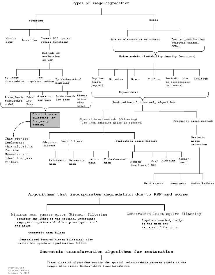
As can be seen from the diagram above, it is important to know that different blur degradations require the use of different PSF (Point Spread Function) mathematical model.
For example, motion blur would require different PSF than say a degradation caused by ripple distortion or by a normal blur degradation. Even blur degradation itself has many different types (motion, lens, Gaussian, Radial, etc...) and different mathematical function for PSF would be needed for each type to obtain an accurate restoration that matches the original image as best as possible. For instance, degradation by motion blur, would require a mathematical function for PSF which would take an estimate of the linear or radial motion parameters that caused the blur.
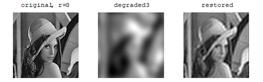
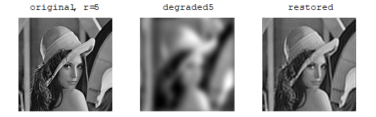
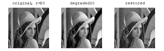
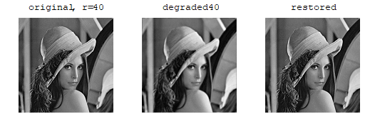
Given the above, and to be able to illustrate the direct inversion algorithm, I had to assume a certain PSF model. I have selected to use the 2D Gaussian low pass filter and the 2D ideal low pass filter. Using these filters, I will start by generating a number of degraded images from an original single undegraded image. I will use different standard deviation values for the Gaussian for each generation of a degraded image, and different radius values for the ideal low pass filter.
In this case, the standard deviation used for the Gaussian is nothing but the radius as well. The radius is measured as the number of pixels from the center or the spectrum. In all cases, the 2D spectrum will be centered in the middle of the image.
After degrading the original image, I will then restore these images using the inverse filtering algorithm and compare the result with the original, undistorted image. I will observer how using different radius values affect the restoration quality, and will compare visually each restored image to the original image and comment on the quality of the restoration.
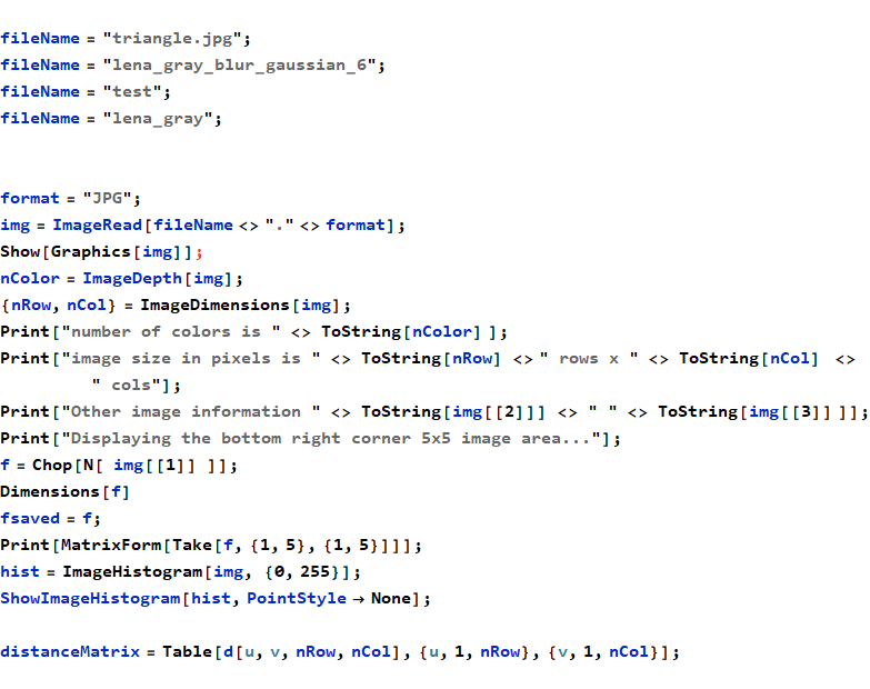
The standard image of Lena will be used throughout this evaluation. It is a gray level, 512 x 512 pixels image that I downloaded from the internet. I have used a gray level image to simplify the implementation, otherwise I would have to perform 2D fourier transformation and inverse transformation on each of the 3 channels. For the purpose of illustrating the algorithm, I did not feel this would not have adding any more value.
The restoration algorithm can be implemented completely in the spatial domain if needed. However, since the algorithm requires performing a convolution operation, and since convolution in the spatial domain is equivalent to multiplication in the frequency domain, we will start by transforming the input image to the frequency domain to take advantage of the speed of the FFT (Fast Fourier Transforms).
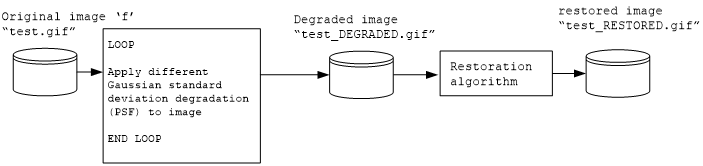
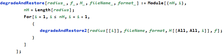
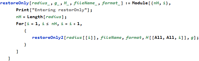
In this implementation, an image is read, degraded using the PSF, and then restored using the direct inversion algorithm. Both the degraded and restored images are saved to disk.
The name of the output image file will be the same as the input image file, but with the word _RESTORED and _DEGRADED appended to the file name. The type of the images outputted will be in the same graphic format as the input image.
This diagram below illustrates the data flow of the program as a black box
A small note on how this report was written
This report was itself written in Mathematica in the same file as the program itself. This made it easier to add comments on the program and have these as part of the report itself as the same time. This feature is attractive since it eliminates the need to separate the program from the documentation or the report as would be the case in other systems.
Project Details
Mathematical model of image degradation
The algorithm is based on the following mathematical model of image degradation.
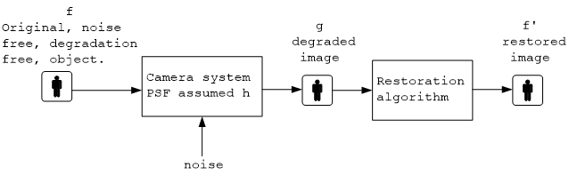
Let the degraded image be called g. Let the camera PSF (point spread function) be called h (This is the degradation function which depends on the system itself, i.e. the camera). Let noise introduced into the degraded image be called η. Let the original, undegraded image be called f.
The degraded image is now given by
g(x,y)=h(x,y)⊗ f(x,y) + η(x,y)
Where the operator ⊗ is the convolution operator.
Taking the 2D fourier transform results in
G(u,v)=H(u,v) F(u,v) + N(u,v)
In this implementation we assume that noise is zero. This results in the following relation
G(u,v)=H(u,v) F(u,v)
Hence,

Now, to obtain the restored image, we perform a 2D inverse fourier transform, let the restored image be 
 = Inverse_2D_Fourier_Transform ( F(u,v) )
Notice that  ) (the restored image) will not be exactly the same as f(x,y) for the following reasons
1. We do not know exactly what the camera PSF function is, we will assume here that the PSF is a 2D Gaussian
filter with a certain standard deviation or an ideal low pass filter.
2. We did not model the noise in this implementation. Noise is difficult to model and depends on many factors.
The following diagram illustrates this process
PSF model
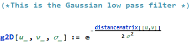
This is the most important function to select for the restoration, since this is how we assume the degradation has occurred in the first place. The following 2D gaussian filter is assumed for the PSF (this is the PSF expressed in the frequency domain)
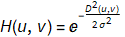
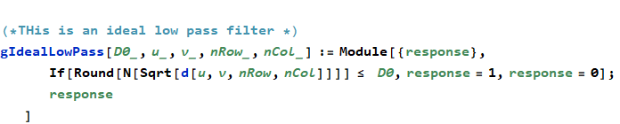
For the low pass filter, we use this definition
 where
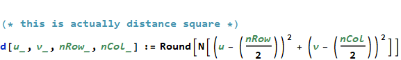
where  is the distance from the center of the spectrum to the point (u,v)
Algorithm steps
The following are the detailed step by step of the algorithm
1. Ask the user for the image file name
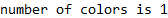
2. Read the image to memory to a matrix f(x,y)
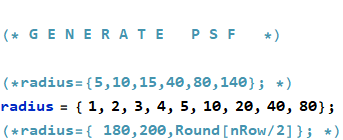
3. Generate N numbers of H(u,v) (PSF) filters (using different Gaussian standard deviations, or different radius values with a fixed increments). For example, use 3,5,10,20,40 pixels. This results in N PSF matrices H(u,v) call them 
4. Do step 3 for both the Gaussian and the Ideal low pass filters.
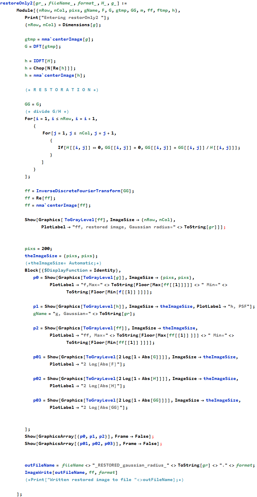
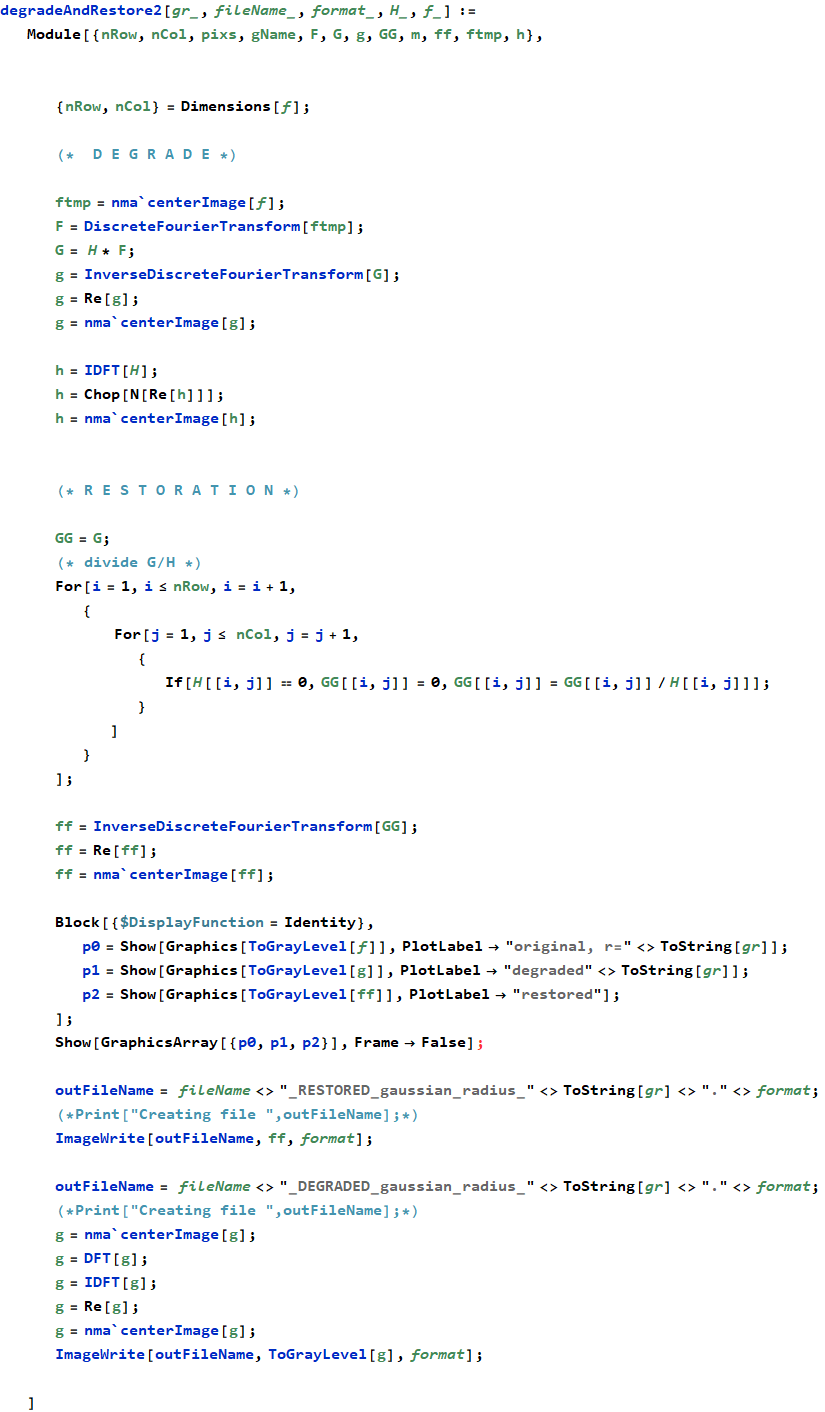
5. Multiply the input image f(x,y) by 
6. Obtain the 2D fourier transform of the original image, call it F(u,v). Due to step 5, this spectrum is now centered.
7. For each PSF H(u,v), generate 2D Fourier transform of a degraded image using 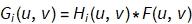
8. For each  generate the spatial image
  by taking the 2D inverse fourier transform.
9. Take the real part of the image generated in step 8.
10. Multiply the result of step 9 by  to get a centered image.
11. Save each of the degraded images  to allow more analysis if needed by external programs such as photoshop.
12. Start the restoration pass. For each  obtain the restored fourier transform
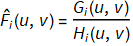
13. For each  apply the 2D IDFT to obtain the restored image
14. Save these images to disk for analysis.
15. Examine visually each of the images  and comment of the quality of restoration by comparing them to the original image f(x,y).
Implementation issues
The main issue to handle in the implementation of the algorithm is the step when we divide 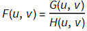 . This is because H can be zero if we use a large standard deviation for the Gaussian. This problem was resolved by explicitly checking for a zero value in the denominator. When this is detected, we set the corresponding value in F(u,v) to 0. This has the effect of setting those high frequencies to zero. Since it is noise that usually occupies the high frequency parts of the image spectrum , this should not cause signification problems in the restoration.
Output, Tables and Results
Conclusions
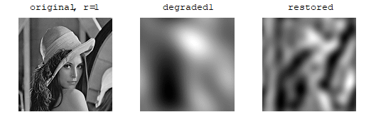
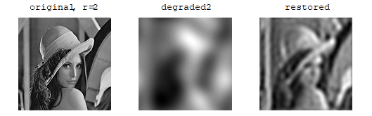
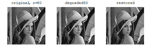
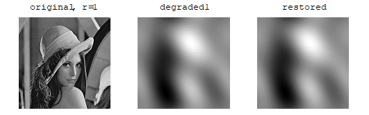
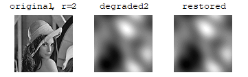
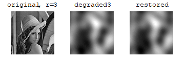
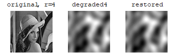
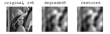
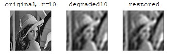
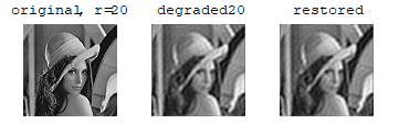
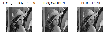
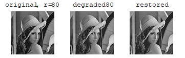
For small radius values, using the Gaussian low pass filter resulted in an acceptable restoration. The ideal low pass filter however produced no restoration that can be detected.
This can be explained by the fact that an ideal low pass filter is not a causal filter and do not occur naturally.
We notice that for a small radius, more image power will be lost in the degradation process, since image power is mostly concentrated in small circles around the center of the 2D spectrum. As the radius is increased, the effect of the restoration decreased until at about radius 100 pixels, there was no restoration that can be noticed.
This project shows that the choice of restoration PSF is critical. It is not possible to use a generic PSF function to restore different degraded images with without having some knowledge of the cause of the degradation to be able to model a PSF which will best restore the image.
If one is able to estimate the PSF, and can ignore the noise, then this algorithm becomes attractive due to its speed when performed in the frequency domain by utilizing the Fast Fourier Transform and due to its simplicity.
Future work and possible extensions to this project
The following are possible options that this work can be expanded on.
1. Investigate other PSF models such as the Butterworth filter.
2. Investigate how to do restoration with the presence of noise by the use of such filters as minimum mean square error (Wiener) or the constrained least square filtering method. These methods are more mathematically complicated, but are considered to produce better restoration results.
3. Investigate the restoration of motion blur.
Sample run and output
Here, I show a complete typical run output of this program. This output will use both the Gaussian and Ideal low pass filters.
Start by initialization of the workspace and loading the needed packages
define the PSF function
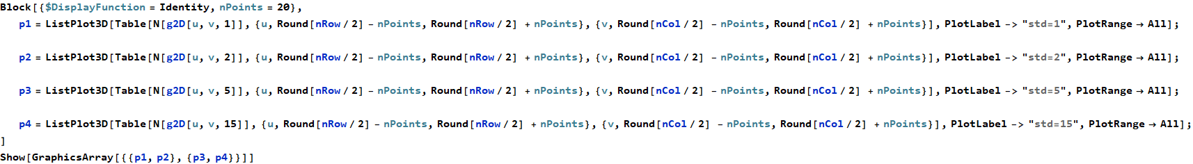
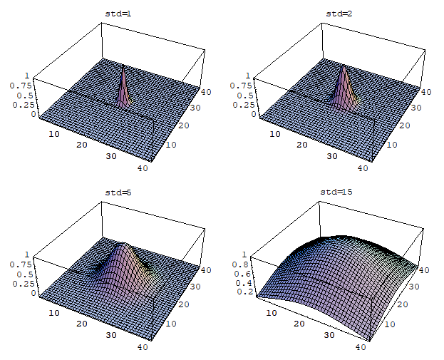
Display PSF using standard deviation of 6 and 40 pixels just for illustration purposes. We will use σ=6 here.
Now, set the working directory to be the same working directory as this note book to allow easy input of
file names for the degraded images.
Now ask the user for the image file name, and read it to memory

sample a 2D continuos gaussian to obtain a discrete version of Gaussian 2D,to use as a filtering window to convolve the image with


Appendix
References
1. Digital Image Processing, second edition, by Gonzalez and Woods
2. Algorithms for image processing and computer vision, by J.R.Parker
3. Lecture notes, EECS 207A by Professor Meyer, UCI Electrical Engineering Department.