This report is a summary of the HIghly constrained Back PRojection (HYPR) team work performed so far relating to the HYPR research project. We will describe the work done and results found.
The goals set for the HYPR project included formulating the HYPR algorithm and some of its variations (such as Wright-Huang HYPR (WH-HYPR), I-HYPR and HYPR-LR) in a mathematical framework which would allow the study and analyze of these algorithms in relation to other well known non-linear methods such as maximum a-posteriori (MAP) estimation and Maximum Likelihood Expectation Maximization (MLEM). These algorithms, like HYPR, use prior information on the object being reconstructed and they are extensively used in nuclear medicine where the data is intrinsically under sampled.
The initial period of this project, which this report reflects on, was spent becoming familiar with the HYPR algorithm and its connection to MLEM. Towards this goal, the HYPR algorithm was formulated mathematically and schematic diagrams created which helped in its implementation. MATLAB simulation software was developed to enable more understanding of the algorithm and its behavior by running it on a number of test cases. Initial comparison between the original HYPR and the WH-HYPR made on a number of different test configuration which are described in detail in the simulation section below. The MLEM algorithm was implemented and compared the HYPR algorithm.
In addition, A mathematical connection between HYPR and Expectation Maximization (EM) is described and formulated.
Please see the appendix for a complete description of the notation used in this section and throrught the rest of the report.
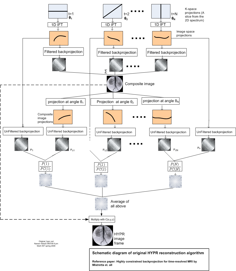
The mathematics of this algorithm will be presented by using the radon transform \(R\) notation and not the matrix projection matrix \(H\) notation.
The projection \(s_{t}\) is obtained by applying radon transform \(R\) on the image \(I_{t}\) at some angle \(\phi _{t}\)
When the original object image does not change with time one can drop the subscript \(t\) from \(I_{t}\) and just write \(s_{t}=R_{\phi _{t}}\left [ I\right ] \)
Next, the composite image \(C\) is found from the filtered back projection applied to all the \(s_{t}\) as follows
Notice that the sum above is taken over \(N\) and not over \(N_{p}\). Next, a projection \(s_{c}\) is taken from \(C\) at angle \(\phi \) as follows
Then the unfiltered back projection 2-D image \(P_{t}\) is generated
And the unfiltered back projection 2-D image \(P_{c_{t}}\) is generated
Then the ratio of \(\frac {P_{t}}{P_{c_{t}}}\) is summed and averaged over the time frame and the result multiplied by \(C\) to generate a HYPR frame \(J\) for the time frame\(.\)Hence for the \(k^{th}\) time frame we obtain
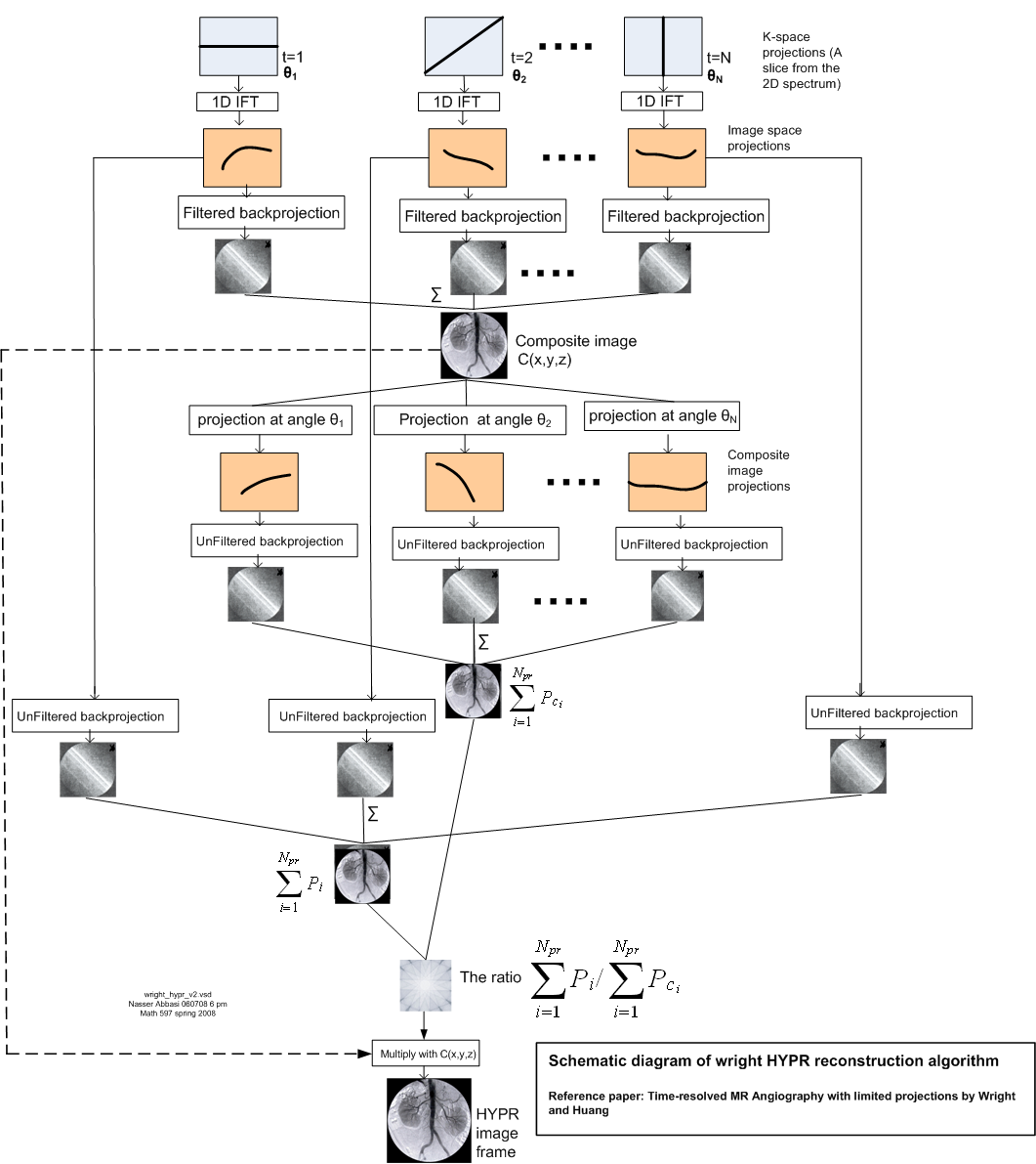
This mathematics of this algorithm will be presented by using the radon transform \(R\) notation and not the matrix projection matrix \(H\) notation.
The projection \(s_{t}\) is obtained by applying radon transform \(R\) on the image \(I_{t}\) at some angle \(\phi _{t}\)
The composite image \(C\) is found from the filtered back projection applied to all the \(s_{t}\)
Notice that the sum above is taken over \(N\) and not over \(N_{p}\). Next a projection \(s_{c}\) is taken from \(C\) at angle \(\phi \) as follows
Then the unfiltered back projection 2-D image \(P_{t}\) is generated
And the unfiltered back projection 2-D image \(P_{c_{t}}\) is generated
Now the set of \(P_{t}\) and \(P_{c_{t}}\) over one time frame are summed the their ratio multiplied by \(C\) to obtain the \(k^{th}\) HYPR frame
The following is a discussion of the Mathematics that connects the MLEM algorithm to HYPR.
According to O’Halloran’s paper[1] the for Maximum-Likelihood Expectation-Maximization (MLEM) algorithm is mathematically equivalent to HYPR. The MLEM algorithm can be used in image reconstruction for medical purposes. Positron Emission Tomography (PET) and Single-Photon Emission Computed Tomography (SPECT) are two types of image reconstruction processes where the MLEM algorithm is used. The purpose here is to show that the MLEM algorithm will work for HYPR reconstructions.
The MLEM algorithm is a process that approximates the solution to
In connection to HYPR, we can view \(H\) as a forward projection matrix, \(\theta \) as the original image being projected and \(g\) the projection produced. The goal is to relate the above matrix based formulation to the radon transform based formulation seen above in the HYPR mathematical section, which is
We formulate the first iteration of the MLEM algorithm based on equation (1) and see how it can be translated into the HYPR process of image reconstruction. The first step of MLEM is
This can be rewritten in matrix form
If we replace \(\frac {1}{z_{n}}\) by \(\frac {1}{\left [ H^{T}\left [ 1\right ] \right ] _{n}}\) in (4), we obtain
The marked portion of the above equation can be viewed as the vector that is produced from unfiltered back projection on the image produced by the ratio
Here the division is done element by element to produce the vector whose elements are the ratios of the respective elements of \(g\) and \(H\hat {\theta }^{\left ( 0\right ) }.\)
In HYPR the equation we want to tie to equation (3) above is as follows
Where the \(\cdot \) represents an element by element multiplication, and the terms in (5) as defined in the section of the HYPR mathematical derivation shown earlier. Hence for (5) and (4) to be equivalent, We must have
Which represents the initial guess for the user image. Therefore, by using for \(\hat {\theta }^{\left ( 0\right ) }\)as an initial guess for the MLEM algorithm the above weighted term of the composite image \(C\), the MLEM algorithm will produce \(\hat {\theta }^{\left ( 1\right ) }\) which is a better approximation to the original image from that of the composite \(C\). And this is what the HYPR algorithm does. It uses the composite image \(C\) to produce the HYPR image \(J\) to approximate the original user image \(I\). Hence a one step of MLEM is equivalent to running HYPR for one time. Therefore, iterative HYPR algorithms can be seen as a multi step application of MLEM.
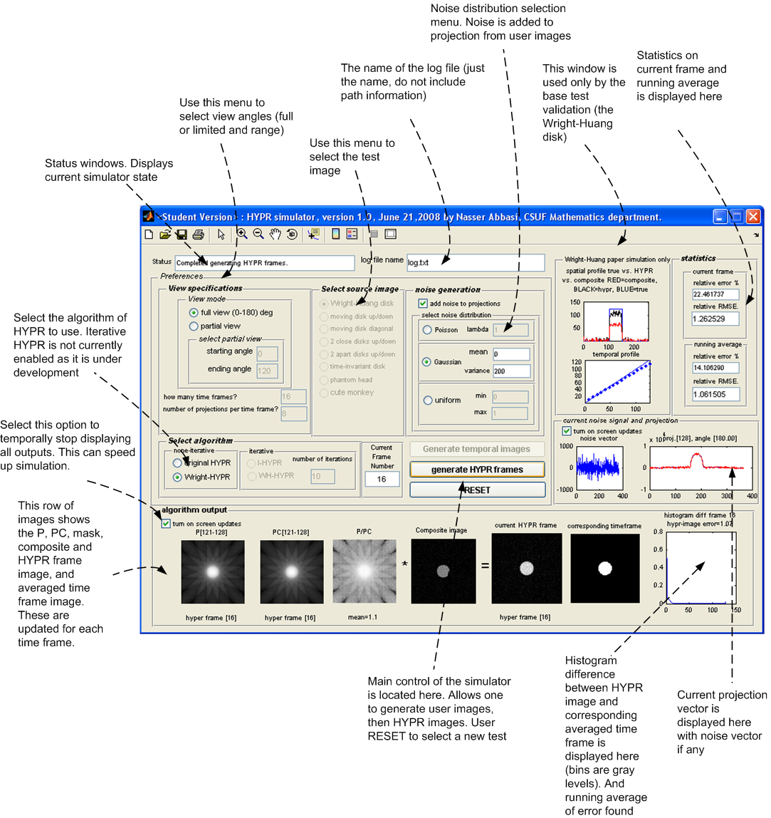
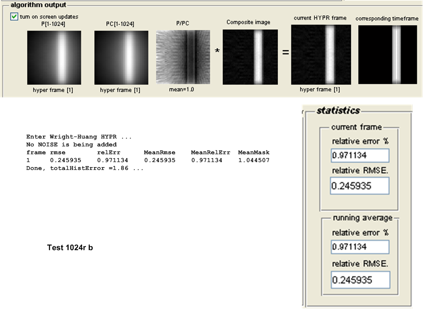
A software simulation written in MATLAB was designed and developed to enable more extensive HYPR testing of different test configurations. The software is GUI based and all test results are saved in a tab-delimited plain text file to allow one further statistical analysis of the data generated by other software. The appendix contains a screen shot of the current version of the simulator (version 1.0).
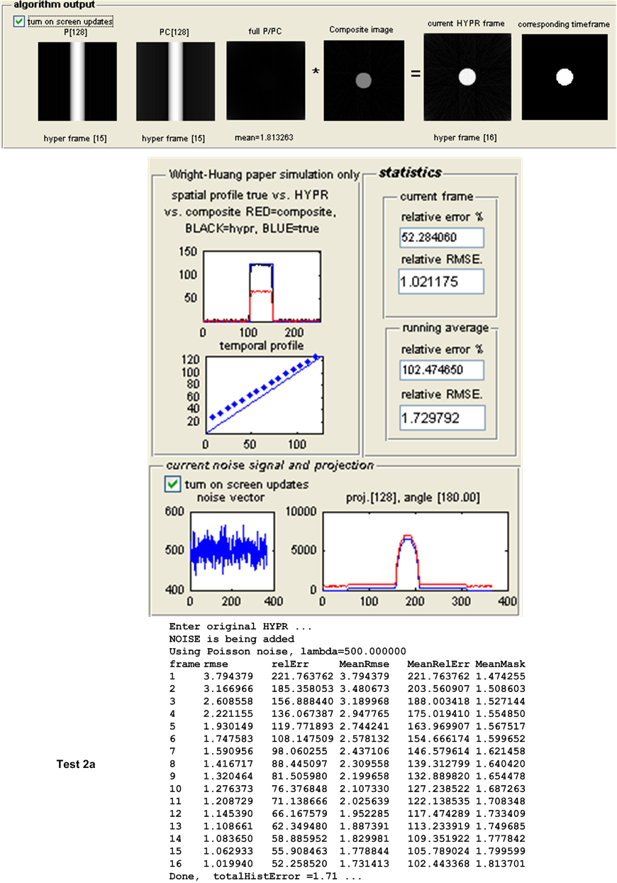
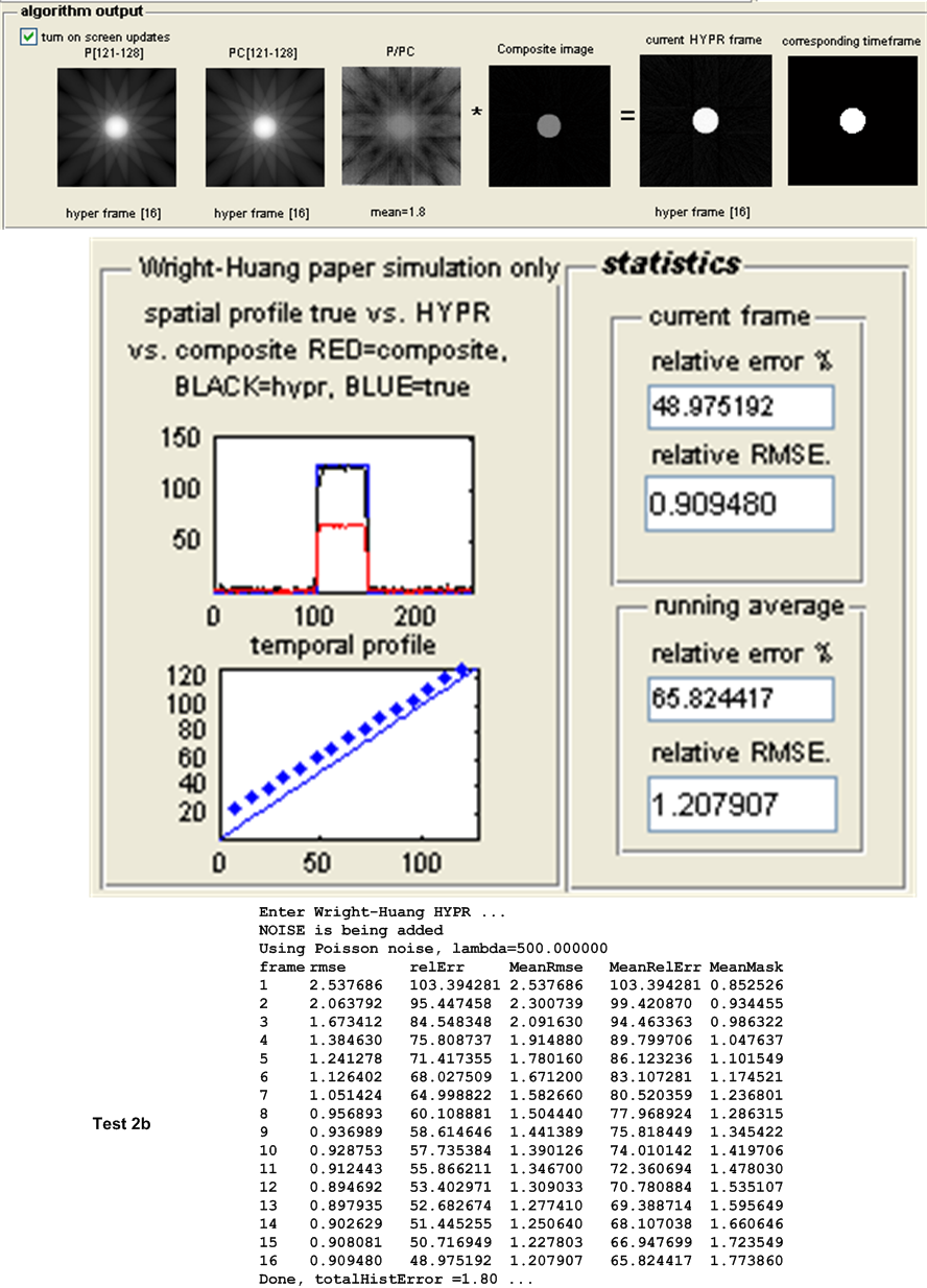
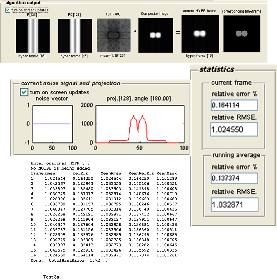
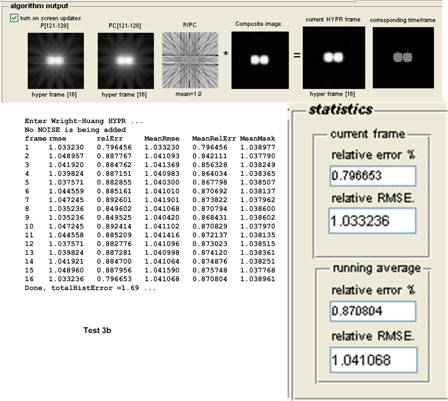
This is a description of the different tests performed. Both the original HYPR and the Wright-Huang HYPR (WH-HYPR) were run and results compared. In the following discussion, we use \(N_{p}\) to mean number of projections in one time frame, and \(N_{w}\) to mean the number of time frames. Hence the total number of projections is \(N_{p}N_{w}\)
The table below describes each test. In this table, a test with the letter ’a’ represents the test being run using the original HYPR and a test with the letter ’b’ represents the test being run using WH-HYPR. Each test was run under both the original HYPR and WH-HYPR.
The first set of tests are designed to detect the effect of Poisson noise on the accuracy of the HYPR algorithm as compared to the WH-HYPR. This was done for different geometry of objects while keeping the number of projections per time frame and the Poisson noise parameter \(\lambda \) fixed.
The second set of tests are designed to detect the effect of Gaussian noise on the accuracy of the HYPR algorithm as compared to the WH-HYPR. This was done for different geometry of objects while keeping the number of projections per time frame and the Gaussian distribution parameters (mean and variance) fixed. The set of tests used here is smaller than the first set due time limitation.
The third set of tests are designed to detect the effect of increasing the number of projections on the accuracy of the HYPR and WH-HYPR. This was done under one fixed configuration and with the absence of noise.
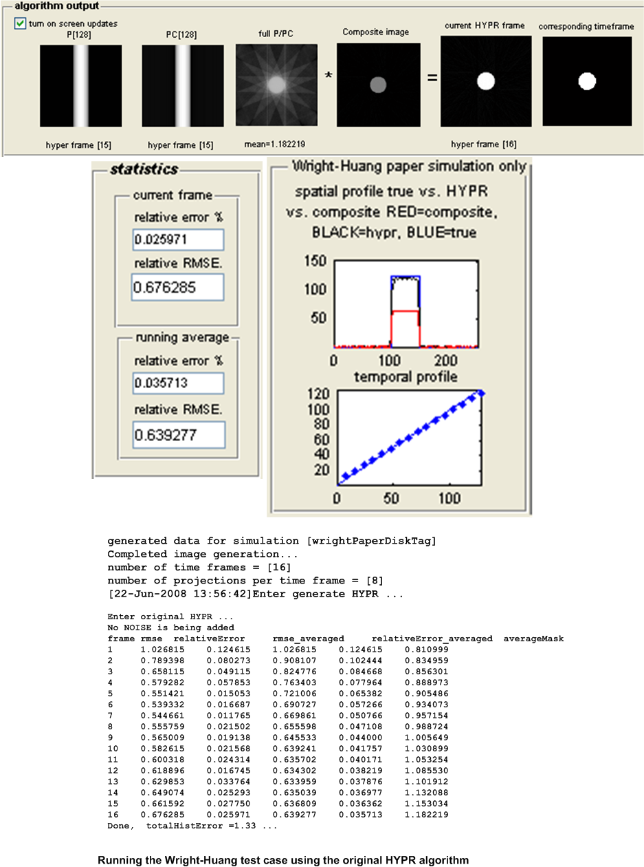
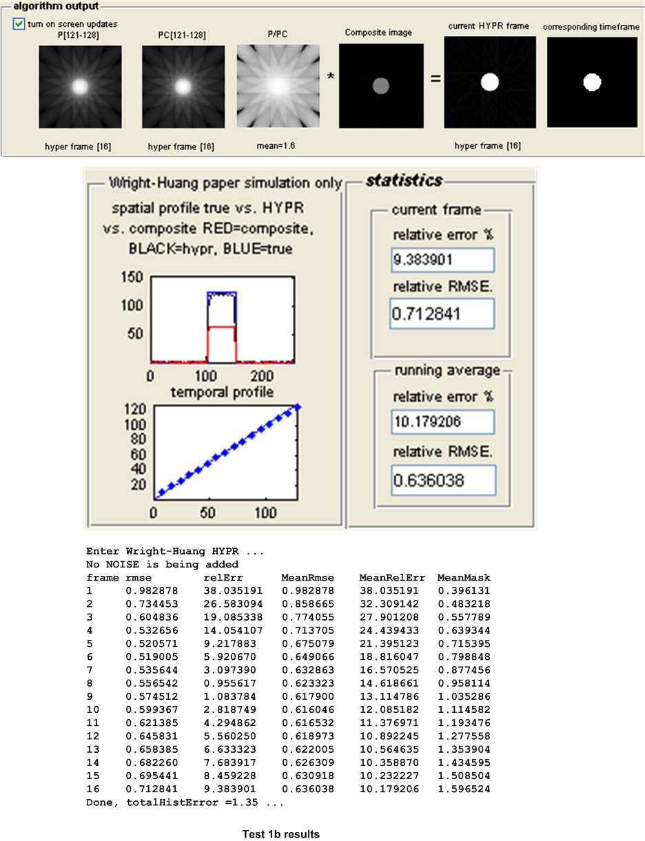
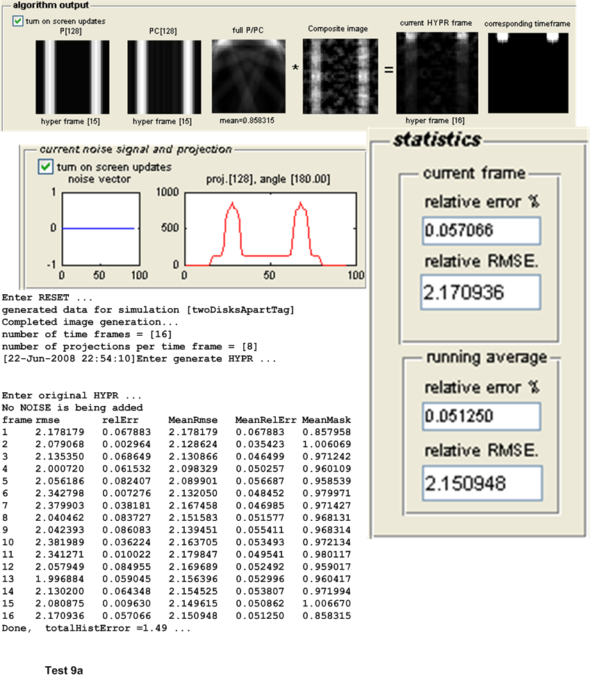
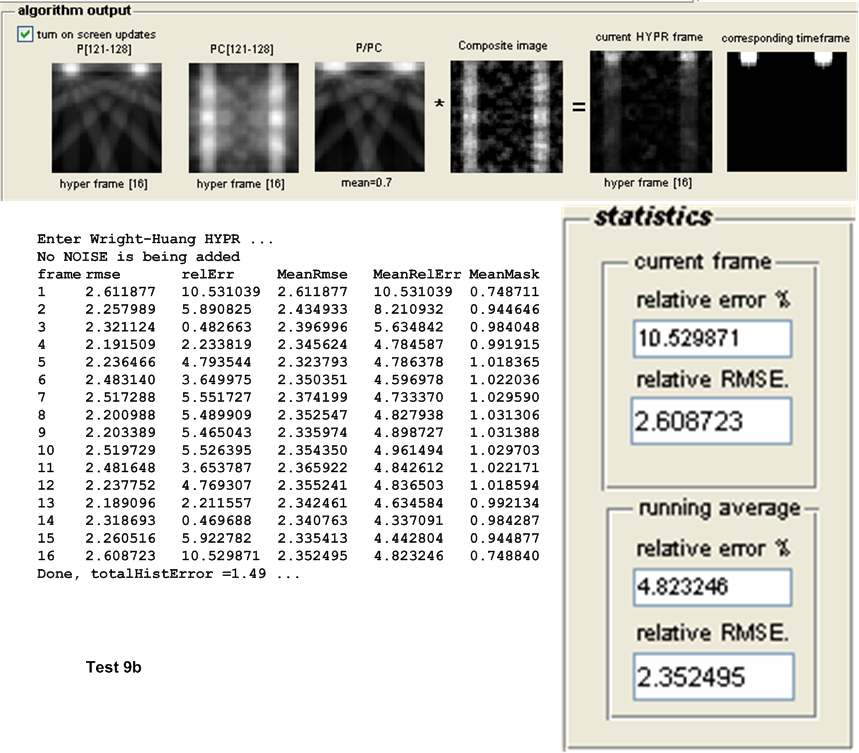
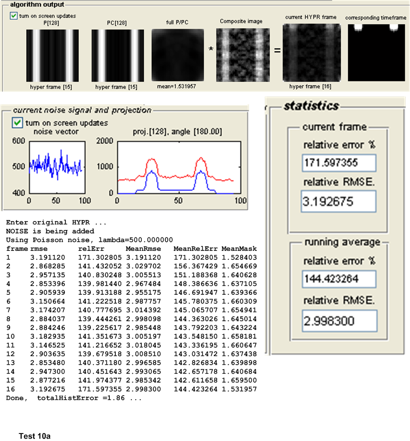
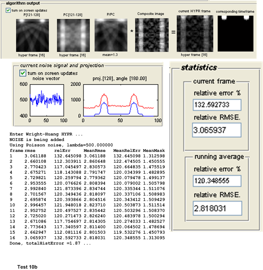
The main measure of accuracy used was relative RMSE. This was calculated as follows: For each HYPR frame image generated, the set of user images which make up the time frame from which the HYPR frame was generated are averaged to obtain an average time frame image. Then the RMSE was obtained between these 2 images as follows: Assuming these are \(N\) total pixels in each image, the error between each corresponding pixels is found as \(H_{i}-I_{i}\) where \(H_{i}\) is a pixel in the HYPR frame image and \(I_{i}\) is the corresponding pixel in the averaged time frame image. This error is then squared. This was done for each pixel. The average of these square values is found, and the square root of the result is found. Hence
This quantity is normalized by dividing it by the mean intensity of the averaged time frame image found earlier. This gives a normalized RMSE value for each time frame generated. When there are more than one time frame generated then the average all these RMSE values are used to obtain one representative value of the RMSE for the test, and that is the value showed in the tables below for the purpose of comparing different tests.
Other statistics are calculated to determine the algorithms accuracy. The relative error between the HYPR image and the averaged time frame is found using the standard formula for relative error. This measure however did not appear to be a good indicator for determining the accuracy of the HYPR image. Another statistical measure used is the histogram difference, which is found as follows. The histogram for each HYPR image frame and the corresponding histogram for the averaged time frame image are calculated and the difference between these histograms found. This measure appear to give a good indication of the performance of each test and correlated well with the RMSE measure used. These results are all written to the log file for further analysis, but are not currently taken into account in the following tests due to time limitation. Only the RMSE measure is currently used to determine the accuracy of the algorithm. The following sections describe each set of tests in more details.
| Test | Test description | ||
| 1a | |||
| 1b | As above, but use the WH-HYPR algorithm. | ||
| 2(a,b) |
|
||
| 3(a,b) |
|
||
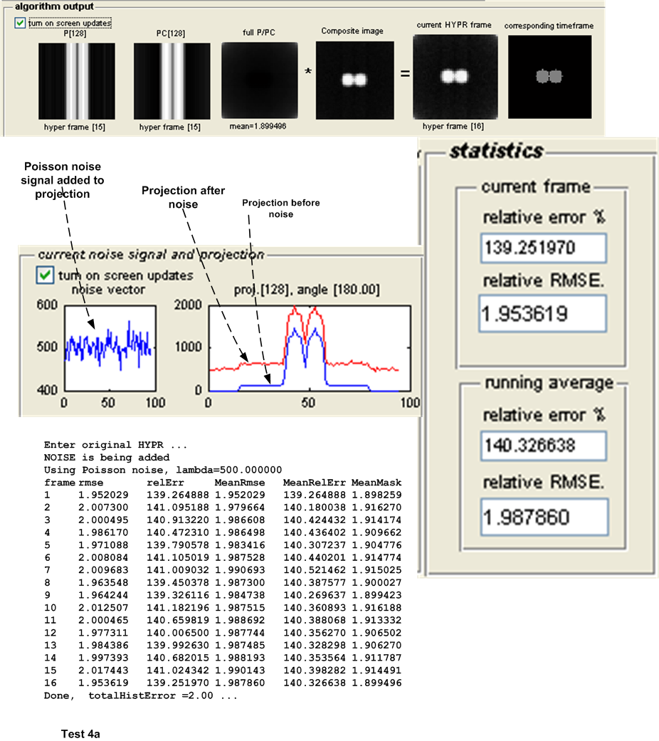
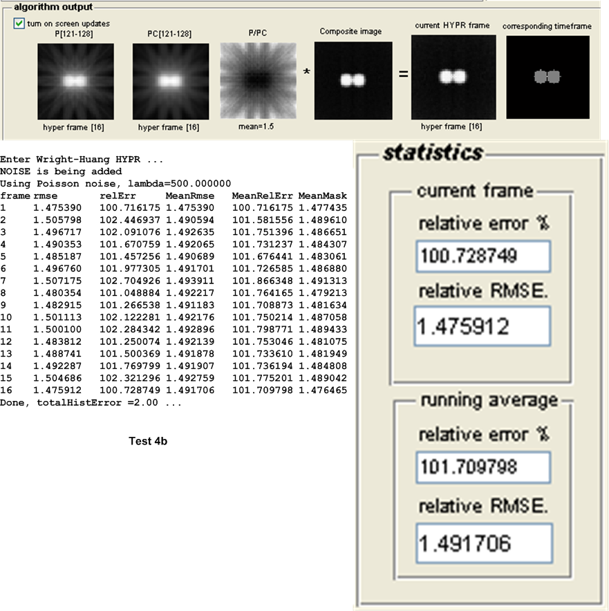
| 4(a,b) | As above, but with Poisson noise with \(\lambda =500\) added to projection \(s\). | ||
| 5(a,b) | Small disk that moves in vertical motion off the center of image. \(N_{p}=8,N_{w}=16\) | ||
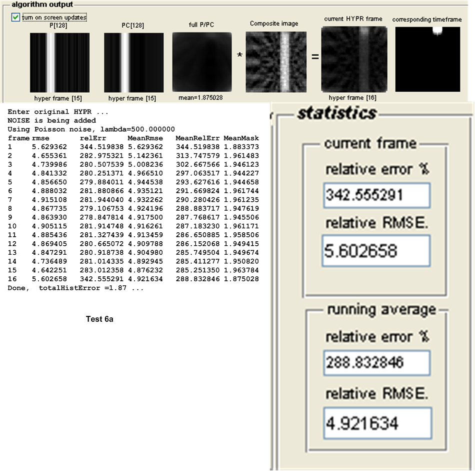
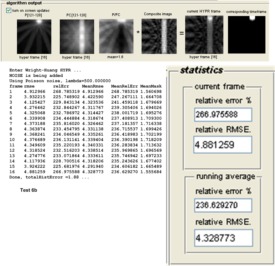
| 6(a,b) | As above, but with Poisson noise with \(\lambda =500\) added to projection \(s\). | ||
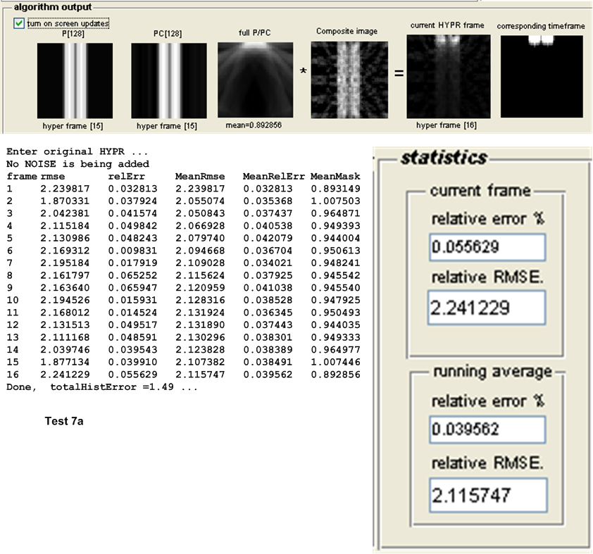
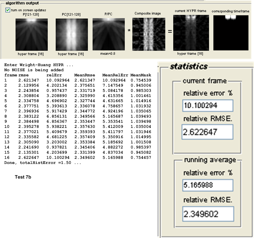
| 7(a,b) | 2 small disks close to each others that move in vertical motion. \(N_{p}=8,N_{w}=16\) | ||
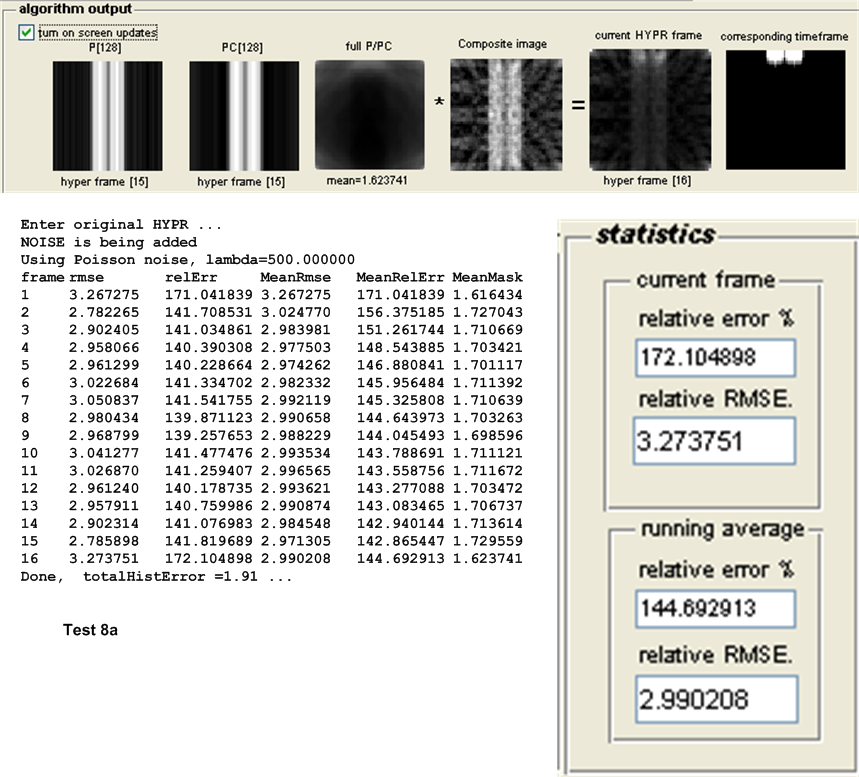
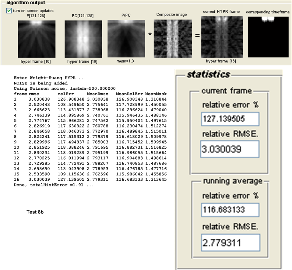
| 8(a,b) | As above, but with Poisson noise with \(\lambda =500\) added to projection \(s\). | ||
| 9(a,b) | 2 small disks further apart from each others that move in vertical motion. | ||
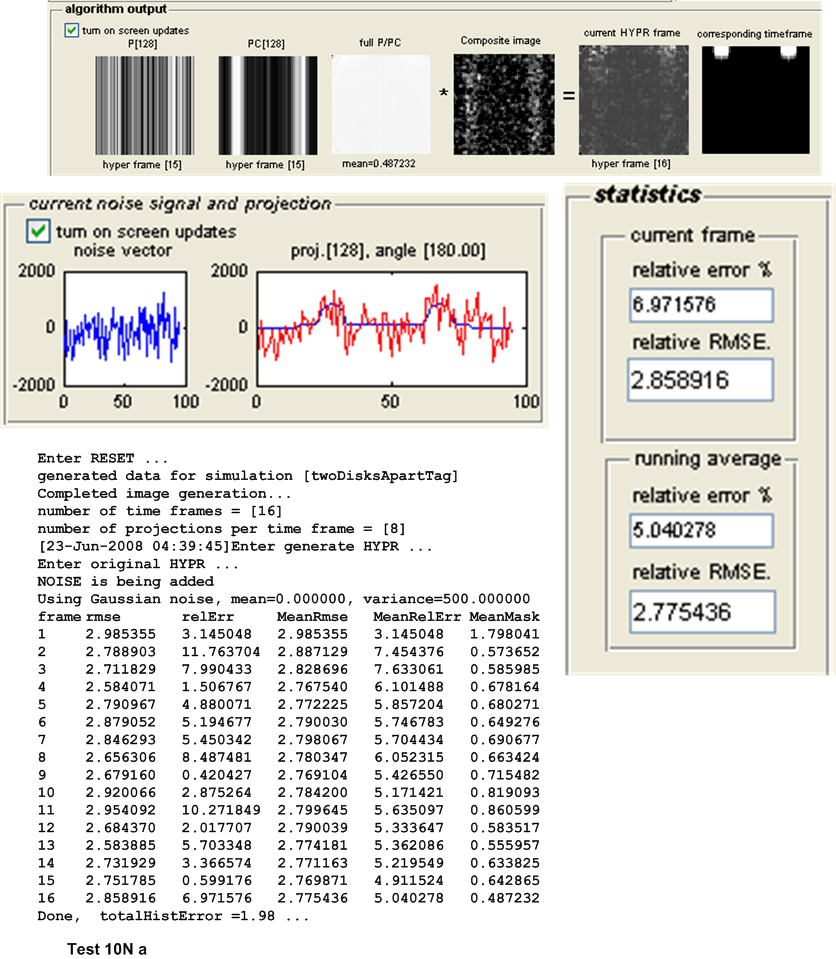
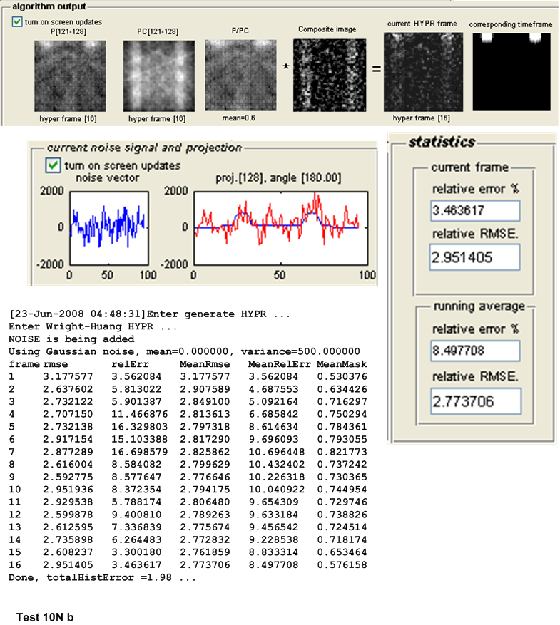
| 10(a,b) | As above, but with Poisson noise with \(\lambda =500\) added to projection \(s\). | ||
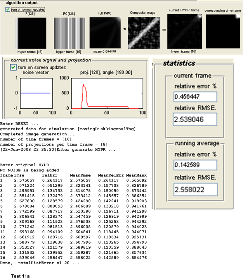
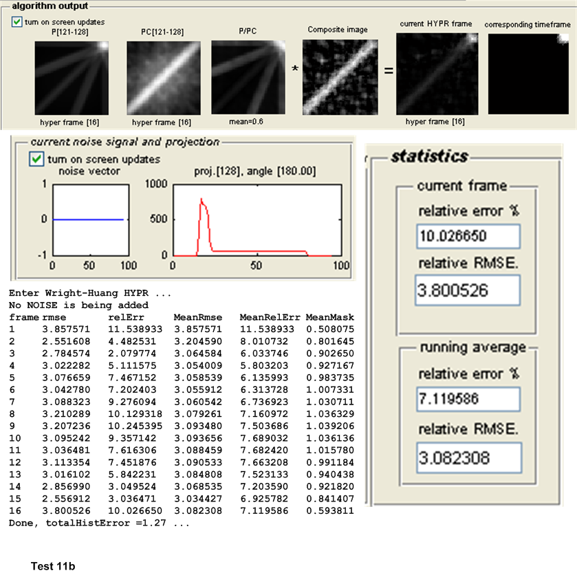
| 11(a,b) | one small disk that move across the image in the diagonal direction. \(N_{p}=8,N_{w}=16\) | ||
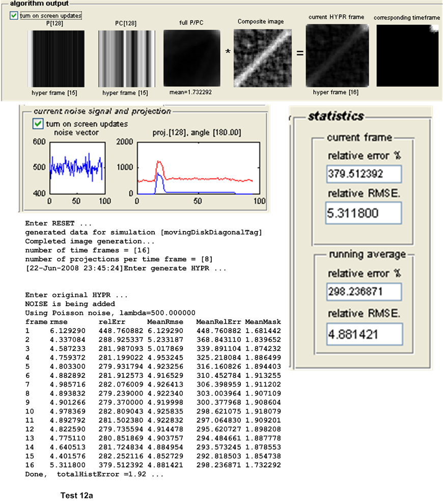
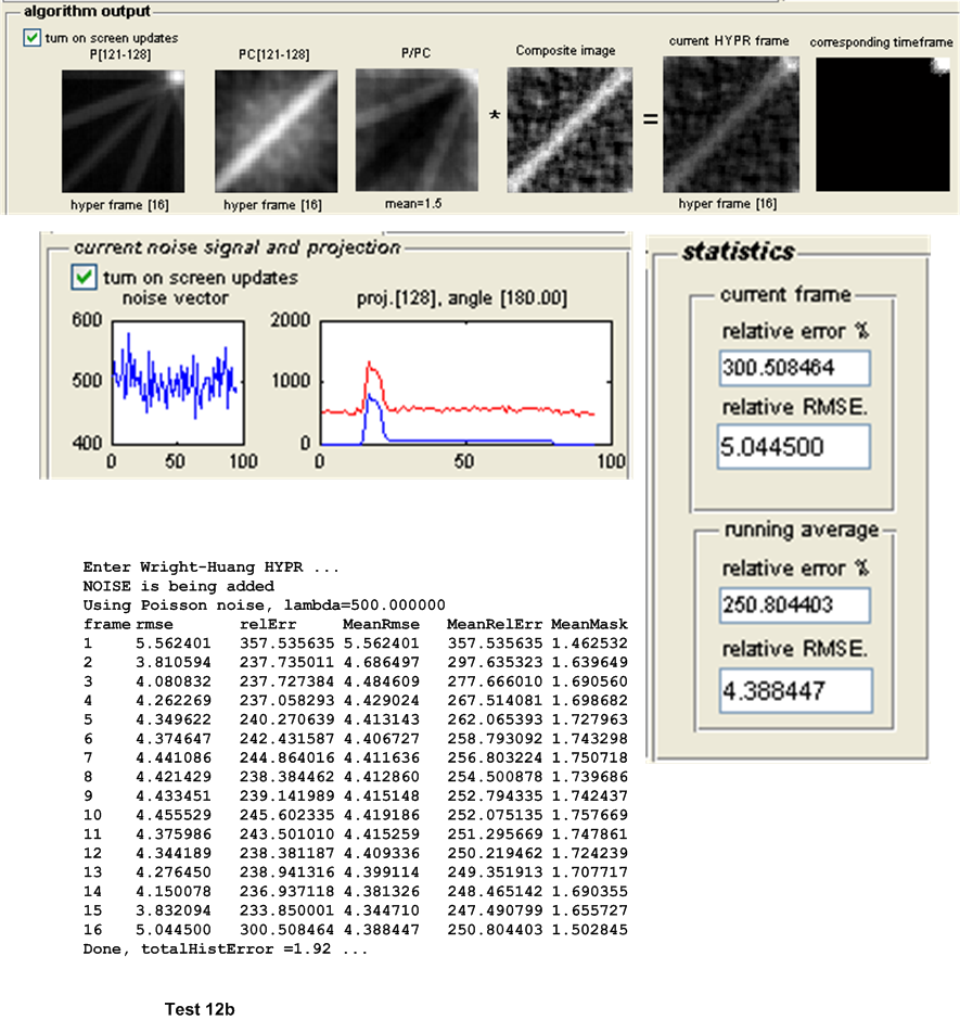
| 12(a,b) | As above, but with Poisson noise with \(\lambda =500\) added to projection \(s\). | ||
The appendix shows the output obtained from the above set of tests. We now present a summary of the results
| Test |
|
|
|
||||||||
| 1 | \(0.639\) | \(0.636\) | WH-HYPR | ||||||||
| 2 (noise) | \(1.7298\) | \(1.2079\) | WH-HYPR | ||||||||
| 3 | \(1.0329\) | \(1.0411\) | Original HYPR | ||||||||
| 4 (noise) | \(1.9879\) | \(1.4917\) | WH-HYPR | ||||||||
| 5 | \(2.6349\) | \(3.095\) | Original HYPR | ||||||||
| 6 (noise) | \(4.9216\) | \(4.3288\) | WH-HYPR | ||||||||
| 7 | \(2.1157\) | \(2.3496\) | Original HYPR | ||||||||
| 8 (noise) | \(2.99\) | \(2.7793\) | WH-HYPR | ||||||||
| 9 | \(2.151\) | \(2.3524\) | Original HYPR | ||||||||
| 10 (noise) | \(2.9983\) | \(2.818\) | WH-HYPR | ||||||||
| 11 | \(2.558\) | \(3.083\) | Original HYPR | ||||||||
| 12 (noise) | \(4.881\) | \(4.3884\) | WH-HYPR | ||||||||
The original HYPR algorithm performed better in each test when noise is absent from projection. This occurs in either time varying or non-time varying configuration. On the other hand, WH-HYPR performed better in each case when noise was present. This occurs in either time varying or non-time varying configuration.
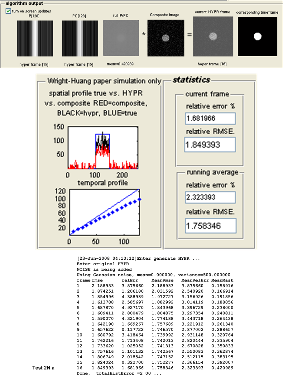
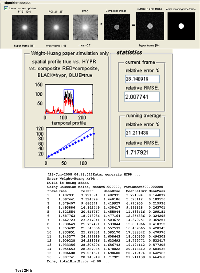
These tests are a repeat of the first set of tests, but with noise generated from normal distribution. Due to time limitation only test 2,6 and 10 described above are repeated since these 3 tests are good representative of the overall tests. The letter N is added to the test name to indicate the use of Normal distribution.
| Test | Test description | ||
| 2N (a,b) |
|
||
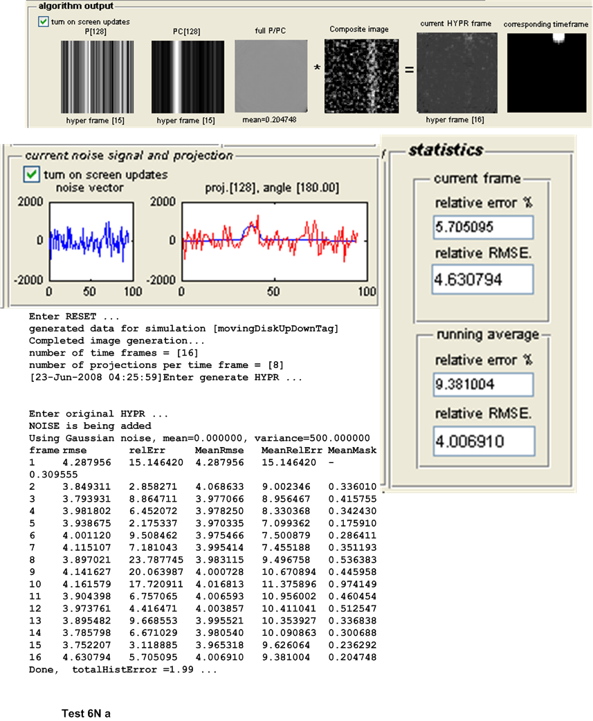
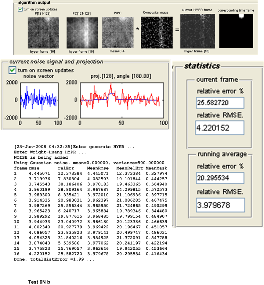
| 6N(a,b) | Repeat test 5, but with the addition of Normal noise with \(\mu =0\) and \(\sigma ^{2}=500\) | ||
| 10N(a,b) | Repeat test 9, but with the addition of Normal noise with \(\mu =0\) and \(\sigma ^{2}=500\) | ||
The appendix shows the output obtained from the above set of tests. Summary of the results is shown below. To clarify the nature of tests below a short description is given again below.
| Test |
|
|
Abs difference |
|
||||||||
| 2N | \(1.7583\) | \(1.7179\) | \(0.0404\) | WH-HYPR | ||||||||
| 6N | \(4.0069\) | \(3.9797\) | \(0.0272\) | WH-HYPR | ||||||||
| 10N | \(2.7754\) | \(2.7737\) | \(0.0017\) | WH-HYPR | ||||||||
WH-HYPR performed better in all 3 cases. This correlated well with results found from the first set of tests where it was observed that WH-HYPR performed better each time Poisson noise was added. In the above 3 tests, normal noise was added and it is observed that WH-HYPR performed better.
As was mentioned earlier, the goal of these tests is to measure the relative accuracy of the algorithms on the same configuration but with increasing number of projections per time frame. It is expected that the accuracy of each algorithm will improve, and we wish to obtain the measure of this improvement as a function of the number of projections per time frame.
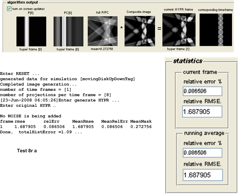
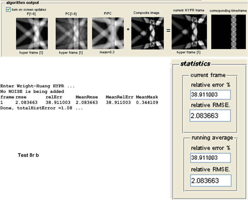
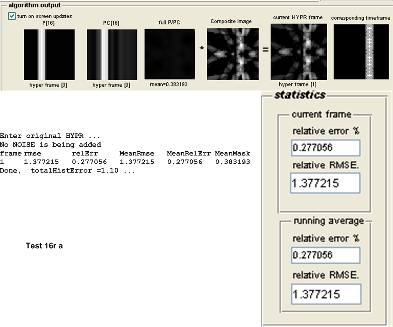
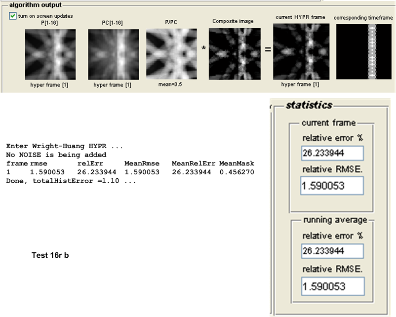
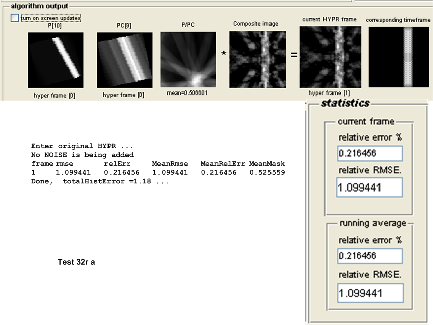
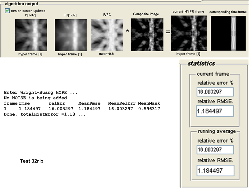
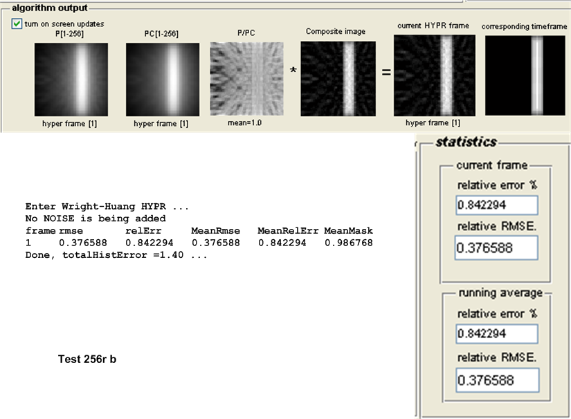
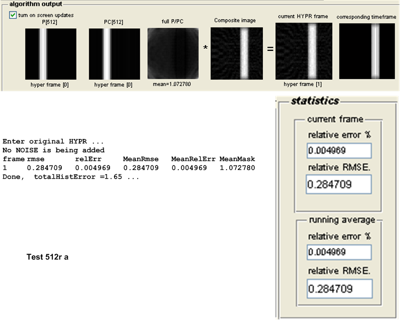
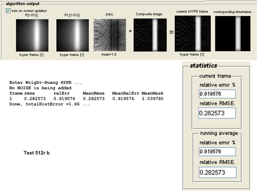
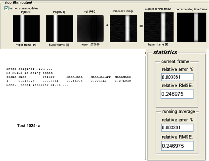
For this purpose, the following test configuration was used: small white disk moving vertically and off center, no noise added. One time frame was used and the following number of projections \(\left \{ 8,16,32,64,128,256,512,1024\right \} \). These tests as named \(8r,16r,32r,128r,256r,512r\) and \(1024r\) respectively. The table below show the result of the tests.
| Test |
|
|
Abs difference |
|
||||||
| \(8r\) | 1.6879 | 2.0836 | 0.3957 | Original HYPR | ||||||
| \(16r\) | 1.3772 | 1.59 | 0.2128 | Original HYPR | ||||||
| \(32r\) | 1.0994 | 1.18845 | 0.0891 | Original HYPR | ||||||
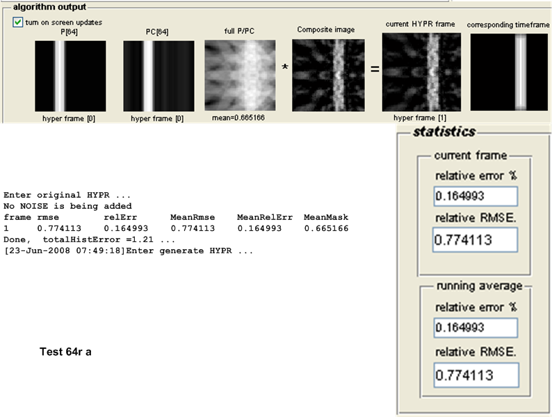
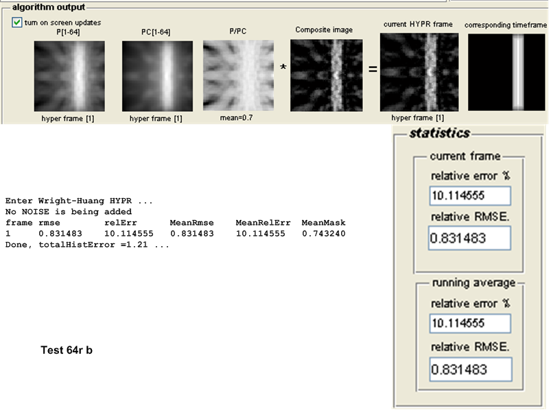
| \(64r\) | 0.774 | 0.8315 | 0.0575 | Original HYPR | ||||||
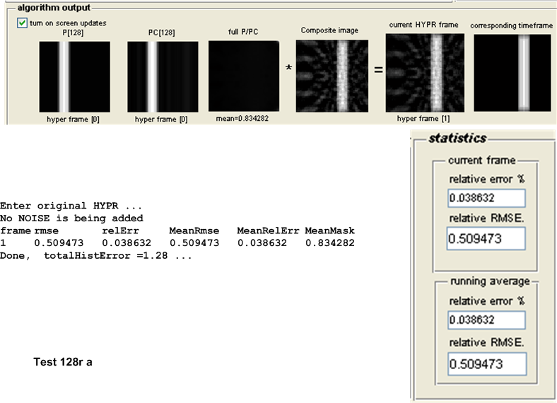
| \(128r\) | 0.5095 | 0.5355 | 0.0260 | Original HYPR | ||||||
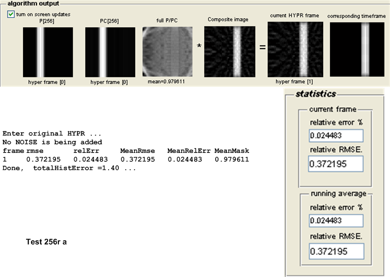
| \(256r\) | 0.3722 | 0.3765 | 0.0043 | Original HYPR | ||||||
| \(512r\) | 0.2847 | 0.2825 | 0.0022 | WH HYPR | ||||||
| \(1024r\) | 0.2469 | 0.2459 | 0.0010 | WH HYPR | ||||||
As the number of projections per time frame increased, the accuracy of WH-HYPR improved. At high number of projections (over 512 per time frame) WH-HYPR bypassed original HYPR and became more accurate. It is not clear at this time if such high number of projections per time frame will conflict with other MRI requirements (sampling rate limitation or other issues), but the above shows that, even with the absence of noise, the WH-HYPR can become more accurate than the Original HYPR but at a cost of having large number of projections per time frame.
Original HYPR performed better than WH-HYPR when the number of projections is relatively low (below 256 per time frame) and when there was no noise present (noise added to projections taken from the original images). This occurred in all configurations (both objects moving in time or fixed).
WH-HYPR performed better when noise is present (both Poisson and Normal noise) and for all number of projections and for all configurations.
In addition, WH-HYPR performed better when there was no noise added, but when the number of projections per time frame was increased.
These results seem to be a direct consequences of the fact that WH-HYPR sums the backprojection images over a time frame period before taking the ratio of these sums in order to obtain the mask image, while in the original HYPR the ratio for each backprojection images is first found and the ratios added and averaged. More analysis will be needed to better understand this difference and to explain mathematically this observed difference between HYPR and WH-HYPR.
Since real MRI data is characterized by low SNR, this leads one to conclude that WH-HYPR should be the preferred choice between these 2 algorithms.
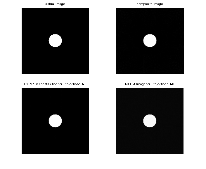
The original HYPR algorithm was compared to 1 step of the MLEM algorithm. A time-invariant white disk with radius \(25\) pixels centered in a \(256\) by \(256\) black image. \(128\) different projection angles were used (ordered using bit-reversed ordering), and the size of the window was set to 8 projections.
The figures below are the actual images produced. The composite image, the HYPR reconstruction for the first HYPR frame, and the corresponding MLEM image. The HYPR and the MLEM images are indistinguishable, although the mean absolute error is slightly higher for HYPR than for MLEM. More detailed comparisons of MLEM and HYPR are planned.