More notes on symbolic features of matlab by Nasser M. Abbasi

This below plots 2 functions on the same figure, giving each curve different color.

>> fplot(inline('x^2-x+3'),[-10:10],'r')

>> hold on;

>> fplot(inline('x^3-x'),[-10:10],'b')

This below finds the factor of a polynomial

>> f=sym('x^4-2*x^3+6*x^2-2*x+5');

>> factor(f)

ans =

(x^2+1)*(x^2-2*x+5)

To expand the above:

>> expand(ans)

ans =

x^4-2*x^3+6*x^2-2*x+5

Find horner representation:

>> horner(f)

ans =

5+(-2+(6+(-2+x)*x)*x)*x

Suppose you want to evaluate an expression for different values, one quick way to do this is to the use the eval command. For example:

>> help eval

EVAL Execute string with MATLAB expression.

EVAL(s), where s is a string, causes MATLAB to execute

the string as an expression or statement.

>> func='x^2+3*y+4*z';

>> x=1; y=3; z=4;

>> eval(func) <--- this use the current values of x,y,z

ans =

>> x=2;

>> eval(func)

ans =

You can use the command ‘numeric’ to numerically the output of ‘solve’ command:

>> f='x^2- 1/x =3'

f =

x^2- 1/x =3

>> solve(f)

ans =

[ 1/2*(4+4*i*3^(1/2))^(1/3)+2/(4+4*i*3^(1/2))^(1/3)]

[ -1/4*(4+4*i*3^(1/2))^(1/3)-1/(4+4*i*3^(1/2))^(1/3)+1/2*i*3^(1/2)*(1/2*(4+4*i*3^(1/2))^(1/3)-2/(4+4*i*3^(1/2))^(1/3))]

[ -1/4*(4+4*i*3^(1/2))^(1/3)-1/(4+4*i*3^(1/2))^(1/3)-1/2*i*3^(1/2)*(1/2*(4+4*i*3^(1/2))^(1/3)-2/(4+4*i*3^(1/2))^(1/3))]

>> numeric(ans)

ans =

1.87938524157182 + 1e-032i

-1.53208888623796 + 3e-032i

-0.347296355333861 - 3e-032i

To work numerically with polynomials:

P=[1 1 –3 –3]

Can be used to represent the polynomial ‘x^3 + x^2 –3x –3’

Notice that p(1) is the coeffient for the largest power of x term. So the order is left to right just as you would write the equation symbolically.

i.e. a3=1; a2=1; a1=-3; a0=-3

To evaluate P at some x do:

x=4;

y=polyval(p,x);

To numerically fit a polynomial over a set of data, use the command polyfit

>> help polyfit

POLYFIT Fit polynomial to data.

POLYFIT(X,Y,N) finds the coefficients of a polynomial P(X) of

degree N that fits the data, P(X(I))~=Y(I), in a least-squares sense.

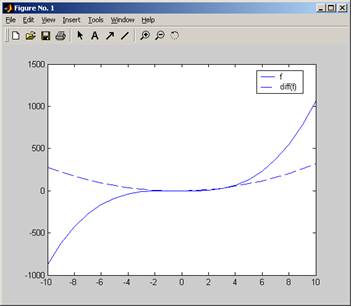
To find the derivative of polynomial

This below shows how to numerically differentiate a polynomial and plot the polynomial and its derivative

>> p=[1 1 -3 -3];

>> pder=polyder(p)

pder =

3 2 -3

>> x=[-10:10];

>> y=polyval(p,x);

>> yder=polyval(pder,x);

>> plot(x,y); hold on; plot(x,yder,'--');

>> legend('f','diff(f)');