Intro to MATLAB symbolic features.
Collected from MATLAB demo
with editing and new additions by Nasser M. Abbasi
% Introduction to the Symbolic Math Toolbox.
% The Symbolic Math Toolbox uses "symbolic
objects" produced
% by the "sym" funtion. For example, the statement
x = sym('x');
% produces a symbolic variable named x.
% You can combine the statements
a = sym('a'); t = sym('t'); x = sym('x'); y =
sym('y');
% into one statement involving the "syms"
function.
syms a t x y
% You can use symbolic variables in expressions and
as arguments to
% many different functions.
r = x^2 + y^2
r =
x^2+y^2
theta = atan(y/x)
theta =
atan(y/x)
e = exp(i*pi*t)
e =
exp(i*pi*t) % Notice that it did not
evaluate numerically this expression since
% one term in it, the ‘t’, is symbolic. Even
though ‘i’ and ‘pi’ are numeric.
% It is sometimes desirable to use the
"simple" or "simplify" function
% to transform expressions into more convenient
forms.
f = cos(x)^2 + sin(x)^2
f =
cos(x)^2+sin(x)^2
f = simple(f)
f =
1
% Derivatives and integrals are computed by the
"diff" and "int" functions.
diff(x^3)
ans =
3*x^2
% Use pretty command to format the output of
symbolic computation to make it easy
% to read
pretty(int(x^3))
4
1/4 x
pretty(int(exp(-t^2)))
1/2
1/2 pi erf(t)
% If an expression involves more than one variable,
differentiation and
% integration use the variable which is closest to
'x' alphabetically,
% unless some other variable is specified as a
second argument.
% In the following vector, the first two elements
involve integration
% with respect to 'x', while the second two are with
respect to 'a'.
[int(x^a), int(a^x), int(x^a,a), int(a^x,a)]
ans =
[ x^(a+1)/(a+1),
1/log(a)*a^x, 1/log(x)*x^a,
a^(x+1)/(x+1)]
% You can also create symbolic constants with the
sym function. The
% argument can be a string representing a numerical
value. Statements
% like pi = sym('pi') and delta = sym('1/10') create
symbolic numbers
% which avoid the floating point approximations
inherent in the values
% of pi and 1/10.
The pi created in this way temporarily replaces the
% built-in numeric function with the same name.
pi = sym('pi')
pi =
pi
delta = sym('1/10')
delta =
1/10
s = sym('sqrt(2)')
s =
sqrt(2)
% Conversion of MATLAB floating point values to
symbolic constants involves
% some consideration of roundoff error. For example, with either of the
% following MATLAB statements, the value assigned to
t is not exactly one-tenth.
t = 1/10, t = 0.1
t =
0.1000
t =
0.1000
% The technique for converting floating point
numbers is specified by an
% optional second argument to the sym function. The possible values of the
% argument are 'f', 'r', 'e' or 'd'. The default is 'r'.
% 'f' stands for 'floating point'. All values are represented in the
% form '1.F'*2^(e) or '-1.F'*2^(e) where F is a
string of 13 hexadecimal
% digits and e is an integer. This captures the floating point values
% exactly, but may not be convenient for subsequent
manipulation.
sym(t,'f')
ans =
'1.999999999999a'*2^(-4)
%'r' stands for 'rational'. Floating point numbers obtained by evaluating
% expressions of the form p/q, p*pi/q, sqrt(p), 2^q
and 10^q for modest sized
% integers p and q are converted to the
corresponding symbolic form. This
% effectively compensates for the roundoff error
involved in the original evaluation,
% but may not represent the floating point value
precisely.
sym(t,'r')
ans =
1/10
% If no simple rational approximation can be found,
an expression of the form
% p*2^q with large integers p and q reproduces the
floating point value exactly.
sym(1+sqrt(5),'r')
ans =
7286977268806824*2^(-51)
% 'e' stands for 'estimate error'. The 'r' form is supplemented by a term
% involving the variable 'eps' which estimates the
difference between the
% thoretical rational expression and its actual
floating point value.
sym(t,'e')
ans =
1/10+eps/40
sym(pi,'e')
ans =
pi-198*eps/359
% 'd' stands for 'decimal'. The number of digits is taken from the
current
% setting of DIGITS used by VPA. Fewer than 16 digits looses some accuracy,
% while more than 16 digits may not be warranted.
digits(15)
sym(t,'d')
ans =
.100000000000000
digits(25)
sym(t,'d')
ans =
.1000000000000000055511151
% The 25 digit result does not end in a string of
0's, but is an accurate
% decimal representation of the floating point number
nearest to 1/10.
% MATLAB's vector and matrix notation extends to
symbolic variables.
n = 4;
A = x.^((0:n)'*(0:n))
A =
[ 1, 1,
1, 1, 1]
[ 1, x,
x^2, x^3, x^4]
[ 1, x^2,
x^4, x^6, x^8]
[ 1, x^3,
x^6, x^9, x^12]
[ 1, x^4,
x^8, x^12, x^16]
D = diff(log(A))
D =
[ 0, 0,
0, 0, 0]
[ 0, 1/x,
2/x, 3/x, 4/x]
[ 0, 2/x,
4/x, 6/x, 8/x]
[ 0, 3/x,
6/x, 9/x, 12/x]
[ 0, 4/x,
8/x, 12/x, 16/x]
% Example to display irrational numbers to an
arbitrary precision
>> vpa(pi,100)
ans =
3.141592653589793238462643383279502884197169399375105820974944592307816406286208998628034825342117068
>> vpa(sqrt(2),100)
ans =
1.414213562373095048801688724209698078569671875376948073176679737990732478462107038850387534327641573
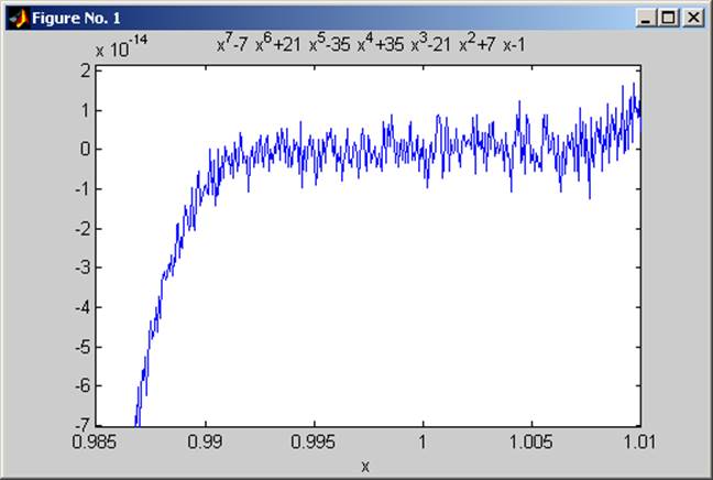
Plotting functions for symbolic expressions:
Ezplot, ezcontour, ezcontourf, ezmesh, ezmeshc,
ezplot3, ezpolar, ezsurf, ezsurfc
>> ezplot('
x^7-7*x^6+21*x^5-35*x^4+35*x^3-21*x^2+7*x-1',[0.985,1.01])
MATLAB commands related to symbolic manipulation
Sym
Syms
subs
SUBEXPR Rewrite in terms of common subexpressions.