and also it will have no Euler acceleration term perpendicular to the radius which
would normally be
and also it will have no Euler acceleration term perpendicular to the radius which
would normally be  . However, there will be Coriolis acceleration due to the point mass changing position
along the radius as the disk spins.
. However, there will be Coriolis acceleration due to the point mass changing position
along the radius as the disk spins.
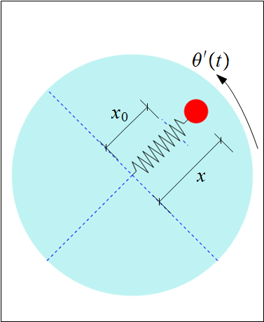
The following diagram shows the physical layout that illustrates the dynamics of a spring mass system on a rotating table or a disk. Mass (the bob) is attached to the end of a spring.
Mass vibrates moving back and forth at the end of a spring that is laid out along the radius of a spinning disk. The bob is considered a point mass. The spring is fixed to the center of the disk which is the origin of the inertial coordinates system. The bob is considered part of the overall disk mass for the purpose of calculation of the mass moment of inertia, therefore the overall mass moment of inertia around the axis of rotation will change as the bob moves along the radius.
There is no friction between the bob and the table. The spring mass is negligible. The spring is assumed to be infinitely rigid against any rotational movement. Hence the spring will move only in the radial direction (as observed in the inerial frame).
In other words, the spring will remain straight all the time no matter how fast the disk spins and how heavy the bob is.
This is important because it means the bob will have no speed component perpendicular to the radius which
would normally be and also it will have no Euler acceleration term perpendicular to the radius which
would normally be . However, there will be Coriolis acceleration due to the point mass changing position
along the radius as the disk spins.
This causes a Coriolis force which generates a torque on the disk. This torque however will change in value as the bob moves and the net effect is that the angular momentum of the overall system remain constant as will be shown below.
The equations of motion for the bob and the disk are derived using both Newton's and Lagrangian methods. It is a good practice to start the analysis by making a velocity, acceleration and force diagrams. The velocity and acceleration diagrams of the system are given below
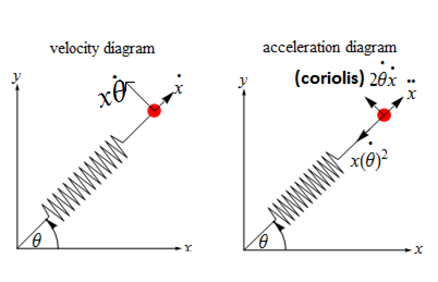
The force diagram is
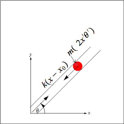
The force  is the spring force on the bob mass.
There will be a reaction force at the center of the disk equal to this force where the spring is attached. But this reaction force produces no torque on the disk since its arm length is zero.
For the bob, applying  along the only degree of freedom the bob can move along, which is the radius
of the disk gives
along the only degree of freedom the bob can move along, which is the radius
of the disk gives
Now  is applied to the disk (and remembering to include the bob mass as part of the disk) in order
to obtain the equation of motion for the
is applied to the disk (and remembering to include the bob mass as part of the disk) in order
to obtain the equation of motion for the  degree of freedom.
The torque is due to the Coriolis acceleration. The Coriolis force  and the distance from the
origin is
and the distance from the
origin is  , hence the toque is
  (the minus sign due to the direction of the torque being clockwise).
Therefore
(the minus sign due to the direction of the torque being clockwise).
Therefore  gives
gives

Hence
 | (2) |
The above 2 equations are now solved numerically for  and
and 
The Lagrangian  is first determined, where
  is the overall kinetic energy of the system and
  is
the overall potential energy of the system.
is
the overall potential energy of the system.

and

Hence

The  motion gives

Hence

which is the same as equation (1) found using Newton's method. Now for the  motion

Hence

which is the same as equation (2) found using Newton's method. Now for the  motion.
It is important to verify that the angular momentum remain constant based on the above model. The angular
momentum must be constant since there are no dissipative forces and no external forces. The initial
angular momentum is given by  where
where  is the initial position of
the bob and
is the initial position of
the bob and  is the initial angular velocity given to the disk. Let
  be the value of this
initial angular momentum. Hence at any point of time in the future the following relation must
hold
be the value of this
initial angular momentum. Hence at any point of time in the future the following relation must
hold

Now, taking derivative with time of the above gives

Which is the same equation of motion for  found above using Newton's and Lagrangian methods. Hence
the assumption that the angular momentum remain constant leads to the equation of motion. This shows that
the angular momentum being constant does not contradicts the assumptions used to derive the equations of
motion.
found above using Newton's and Lagrangian methods. Hence
the assumption that the angular momentum remain constant leads to the equation of motion. This shows that
the angular momentum being constant does not contradicts the assumptions used to derive the equations of
motion.
The equations of motion are solved numerically. At the end of integration step, the new angular momentum is
calculated and was verified that it remained equal to 
Using Mathematica, it is not required to convert the equations to first order, and equations (1) and (2) can be given to NDSolve as is. The following is an example showing how this was done. In this example, the following initial conditions and parameters are used
 meter
meter kg
kg N/m
N/m kg
kg meter
meter rad/sec.
The equations are solved and  and
and  are plotted. This was done for
  seconds
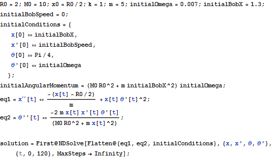
The plots are
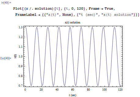
and
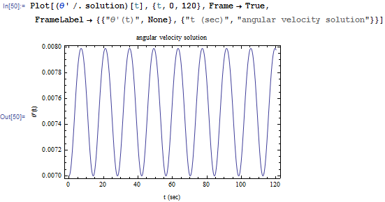
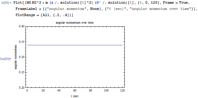
To verify that the angular momentum is conserved, it is calculated and plotted as well. The result shows it is constant. This verifies that the numerical solution is correct.