Solve the 2-D Laplace PDE for a rectangular plate with Dirichlet boundary conditions

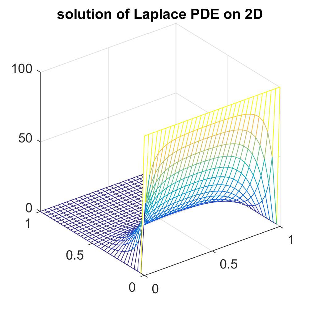
Problem: Solve \(\nabla ^{2}T\left (x,y\right )=0\) on the following plate, with height \(h=30\), and width \(w=10\), and with its edges held at ﬁxed temperature as shown, ﬁnd the steady state temperature distribution

Mathematica NDSolve[] does not currently support Laplace PDE as it is not an initial value problem.

Jacobi iterative method is used below to solve it. 100 iterations are made and then the resulting solution plotted in 3D.

Mathematica

n = 32;  (*grid size*) 
h = 1/(n-1);(*grid spacing*) 
u = Table[0.,{n},{n}]; (*init to zero*) 
u[[1,All]] = 100; (*B.C.*) 
 
Do[ (*iterate 100 times*) 
  tmp=u; 
  For[i=2,i<=n-1,i++, 
    For[j=2,j<=n-1,j++, 
      tmp[[i,j]]= 
        (1/4)(u[[i-1,j]]+u[[i+1,j]]+ 
           u[[i,j-1]]+u[[i,j+1]]) 
    ] 
  ]; 
 
  u=tmp, 
  {100} 
]; 
 
ListPlot3D[u,PlotRange->All, 
 ImagePadding->20, 
 Mesh->{n,n}, 
 ImageSize->300, 
 PlotLabel->"solution of Laplace PDE on 2D" 
]

pict

Matlab

n = 32; 
h = 1/(n-1); %grid spacing 
u = zeros(n,n); 
u(1,:) = 100; %B.C. 
 
% coordinates 
[X,Y]  = meshgrid(0:h:1,0:h:1); 
 
for k=1:100 
    tmp = u; 
 
    for i=2:n-1 
        for j=2:n-1 
          tmp(i,j)=... 
           (1/4)*(u(i-1,j)+u(i+1,j)+... 
             u(i,j-1)+u(i,j+1)); 
        end 
    end 
 
    u=tmp; 
end 
 
mesh(X,Y,u); 
title('solution of Laplace PDE on 2D'); 
set(gcf,'Position',[10,10,320,320]);

pict

4.2 Solve the 2-D Laplace PDE for a rectangular plate with Dirichlet boundary conditions