
Problem:
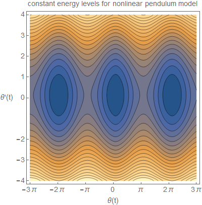
Plot the constant energy levels for the nonlinear pendulum in \(\theta ,\dot {\theta }\)
Assume that \(m=1,g=9.8m/s^{2},L=10m\)
Answer:
The constant energy curves are curves in the Y-X plane where energy is constant. The Y-axis represents \(\dot {\theta }\), and the X-axis represents \(\theta \)
We assume the pendulum is given an initial force when in the initial position (\(\theta =0^{0}\)) that will cause it to swing anticlock wise. The pendulum will from this point obtain an energy which will remain constant since there is no damping.
The higher the energy the pendulum posses, the larger the angle \(\theta \) it will swing by will be.
If the energy is large enough to cause the pendulum to reach \(\theta =\pi \) (the upright position) with non zero angular velocity, then the pendulum will continue to rotate in the same direction and will not swing back and forth.
The expression for the energy \(E\) for the pendulum is first derived as a function of \(\theta ,\dot {\theta }\)\begin {align*} E & =PE+KE\\ & =mgL\left ( 1-\cos \theta \right ) +\frac {1}{2}mL^{2}\dot {\theta }^{2} \end {align*}
The school PDF report contains more information on this topic.
This was solved in Mathematica using the ListContourPlot[] command after generating the energy values.
The original Matlab implementation is left below as well as the Maple implementation. However, these were not done using the contour method, which is a much simpler method. These will be updated later.
The following is the resulting plot for \(m=1,g=9.8m/s^{2} ,L=10m\)
Mathematica
SetDirectory[NotebookDirectory[]];
energy[theta_, speed_, m_, g_, len_] := m*g*len*(1 - Cos[theta]) + (1/2)*m*len^2*speed^2;
m = 1; g = 9.8; len = 10;
data = Table[energy[i, j, m, g, len], {j, -4, 4, 0.01}, {i, -3*Pi, 3*Pi, Pi/20.}];
ListContourPlot[data, InterpolationOrder -> 2, Contours -> 20, MaxPlotPoints -> 30,
  DataRange -> {{-3*Pi, 3*Pi}, {-4, 4}},
  FrameTicks -> {{{-4, -3, -2, 0, 1, 2, 3, 4}, None},
    {{-3*Pi, -2*Pi, -Pi, 0, Pi, 2*Pi, 3*Pi}, None}},
  FrameLabel -> {{"\[Theta]'(t)", None},
    {"\[Theta](t)", "constant energy levels for nonlinear pendulum model"}}, ImageSize -> 400,
  LabelStyle -> 14, RotateLabel -> False]
Matlab
function HW2
%HW2 problem. MAE 200A. UCI, Fall 2005
%by Nasser Abbasi

%This MATLAB function generate the constant energy level
%curves for a nonlinear pendulum with no damping

close all; clear;
m=1; g=9.8; L=10;

%number of data points (positio vs speed) to find per curve
nPoints=40;

nEnergyLevels = 8; %number of energy levels
lowAnglesToVisit = linspace(0,pi,nEnergyLevels);
lowEnergyLevels(1:nEnergyLevels)=m*g*L*(1-cos(lowAnglesToVisit));
highAnglesToVisit = linspace(pi,2*pi,2*nEnergyLevels);
highEnergyLevels=zeros(1,2*nEnergyLevels);

initialHighEnergy=2*m*g*L;
Q=0.2;
for i=1:2*nEnergyLevels
  highEnergyLevels(i) = initialHighEnergy+(Q*i*initialHighEnergy);
end

A = zeros(length(lowAnglesToVisit)+length(highAnglesToVisit),2);
A(:,1) = [lowAnglesToVisit highAnglesToVisit];
A(:,2) = [lowEnergyLevels highEnergyLevels];

[nAngles,~]=size(A);
data=zeros(nPoints,2);

for j=1:nAngles

    currentAngle=A(j,1);
    currentEnergyLevel =A(j,2) ;
    angles=linspace(0,currentAngle,nPoints);
    data(1:nPoints,1)=angles(:);

    for m=1:nPoints
        data(m,2)=speed(currentEnergyLevel,angles(m));
    end
    doPlots(data);
end

title(sprintf(['constant energy curves, nonlinear pendulum,'...
               'quantum=%1.3f'],Q));
xlabel('angle (position)');
ylabel('speed');
set(gca,'xtick',[-4*pi,-3*pi,-2*pi,-pi,0,pi,2*pi,3*pi,4*pi]);
set(gca,'XTickLabel',{'-4pi','-3pi','-2pi','-pi',...
                      '0','pi','2pi','3pi','4pi'})

print(gcf, '-dpdf', '-r600', 'images/matlab_e77_1');

function s=speed(energy,angle)
m=1; g=9.8; L=10;
if angle<pi
    s=sqrt(2/(m*L^2)*(energy-m*g*L*(1-cos(angle))));
else
    s=sqrt(2/(m*L^2)*(energy-m*g*L*(1+cos(angle-pi))));
end

function doPlots(data)
plotCurves(data,0);
plotCurves(data,2*pi);
plotCurves(data,-2*pi);

function plotCurves(data,k)
plot(data(:,1)+k,data(:,2));
hold on;
plot(data(:,1)+k,-data(:,2));
plot(-data(:,1)+k,-data(:,2));
plot(-data(:,1)+k,data(:,2));

Maple
The Maple solution was contributed by Matrin Eisenberg
 restart;
 plotEnergyLevels:= proc(m::positive, g::positive, L::positive, Erange::positive, numContours::posint)
   local plotOptions, maxTheta, thetaDot, plotContour, Emax, energies, contours;
   plotOptions := args[6..-1];
   maxTheta := E- arccos(max(1-E/m/g/L, -1));
   thetaDot := E- theta- sqrt(max(2/m/L^2 * (E - m*g*L*(1-cos(theta))), 0));
   plotContour := E- plot(thetaDot(E), 0..maxTheta(E), numpoints=5, plotOptions);

   # Create first quadrant of middle region of the graph.
   Emax := Erange*m*g*L;
   energies := {Emax * n/numContours $ n=1..numContours};
   if Erange  2 then energies := energies union {2*m*g*L}; fi;
   contours := map(plotContour, energies);

   # Create other quadrants.
   map2(rcurry, plottools[reflect], {[[0,0],[0,1]], [0,0], [[0,0],[1,0]]});
   contours := contours union map(f- map(f, contours)[], %);

   # Create left and right regions of the graph.
   map2(rcurry, plottools[translate], {-2*Pi,2*Pi}, 0);
   contours := contours union map(f- map(f, contours)[], %);

   # Complete the graph.
   plots[display]([%[], plot([[-2*Pi,0], [0,0], [2*Pi,0]], plotOptions, style=point)],
     view=[-3*Pi..3*Pi, -thetaDot(Emax)(0)..thetaDot(Emax)(0)],
     title="Constant energy levels, undamped pendulum",
     labels=["angle", "angular speed"],
     xtickmarks=[seq](evalf(k*Pi)=sprintf("%a pi", k), k=-3..3));
 end:
 plotEnergyLevels(1, 9.8, 10, 5, 15);


;

sectionSolve numerically the ODE u””+u=f using point collocation method
Problem: Give the ODE \[ \frac {d^{4}u\left ( x\right ) }{dx^{4}}+u\left ( x\right ) =f \] Solve numerically using the point collocation method. Use 5 points and 5 basis functions. Use the Boundary conditions \(u\left ( 0\right ) =u\left ( 1\right ) =u^{\prime \prime }\left ( 0\right ) =u^{\prime \prime }\left ( 1\right ) =0\)
Use the trial function \[ g\left ( x\right ) ={\displaystyle \sum \limits _{i=1}^{N=5}} a_{i}\left ( x\left ( x-1\right ) \right ) ^{i}\] Use \(f=1\)
The solution is approximated using \(u\left ( x\right ) \approx g\left ( x\right ) ={\displaystyle \sum \limits _{i=1}^{N=5}} a_{i}\left ( x\left ( x-1\right ) \right ) ^{i}\).
\(N\) equations are generated for \(N\) unknowns (the unknowns being the undetermined coefficients of the basis functions). This is done by setting the error to zero at those points. The error being \[ \frac {d^{4}g\left ( x\right ) }{dx^{4}}+g\left ( x\right ) -f \] Once \(g\left ( x\right ) \) (the trial function is found) the analytical solution is used to compare with the numerical solution.
Mathematica
Clear["Global`*"];
nBasis  = 5;
nPoints = 5;
a = Array[v,{nBasis}]
Out[392]= {v[1],v[2],v[3],v[4],v[5]}
trial    = Sum[a[[n]] (x(x-1))^n,{n,1,nBasis}];
residual = D[trial,{x,4}]+trial-1;
mat      = Flatten[Table[residual==0/.x->n/(2*nPoints-1),
             {n,1,nPoints-1}]];

mat = Join[mat,{2 a[[1]]+2a[[2]]==0}];
sol = N@First@Solve[mat,a]
Out[397]= {v[1.]->-0.0412493,
           v[2.]->0.0412493,
           v[3.]->0.000147289,
           v[4.]->-0.0000245233,
           v[5.]->-3.28259*10^-8}
numericalSolution=Chop@
   FullSimplify@Sum[sol[[n,2]](x(x-1))^n,
                   {n,1,nBasis}]

numericalSolutionDiff4 = D[numericalSolution,{x,4}];
numericalMoment = D[numericalSolution,{x,2}];
\begin {equation*} \begin {split} 0.0412493 x-0.0826459 x^3+0.0416667 x^4 -0.00034374 x^5-1.51283*10^-8 x^6\\ +0.0000984213 x^7-0.0000248515 x^8 +1.64129*10^-7 x^9-3.28259*10^-8 x^10 \end {split} \end {equation*}
(*now analytical solution is obtained
using DSolve and compared to numerical solution*)
eq = u''''[x]+u[x]==1;
bc = {u[0]==0,u[1]==0,u''[0]==0,u''[1]==0};
analyticalSolution=First@DSolve[{eq,bc},u[x],x];
analyticalSolution=u[x]/.analyticalSolution;
analyticalSolution=FullSimplify[analyticalSolution]
\[ -\frac {\cos \left (\frac {1-(1+i) x}{\sqrt {2}}\right )+\cos \left (\frac {1-(1-i) x}{\sqrt {2}}\right )+\cosh \left (\frac {1-(1+i) x}{\sqrt {2}}\right )+\cosh \left (\frac {1-(1-i) x}{\sqrt {2}}\right )-2 \left (\cos \left (\frac {1}{\sqrt {2}}\right )+\cosh \left (\frac {1}{\sqrt {2}}\right )\right )}{2 \left (\cos \left (\frac {1}{\sqrt {2}}\right )+\cosh \left (\frac {1}{\sqrt {2}}\right )\right )} \]
analyticalMoment = D[analyticalSolution,{x,2}];
\[ -\frac {-i \cos \left (\frac {1-(1+i) x}{\sqrt {2}}\right )+i \cos \left (\frac {1-(1-i) x}{\sqrt {2}}\right )+i \cosh \left (\frac {1-(1+i) x}{\sqrt {2}}\right )-i \cosh \left (\frac {1-(1-i) x}{\sqrt {2}}\right )}{2 \left (\cos \left (\frac {1}{\sqrt {2}}\right )+\cosh \left (\frac {1}{\sqrt {2}}\right )\right )} \]
dispError[pt_] :=
  ((analyticalSolution-numericalSolution)/.x->pt)/
     (analyticalSolution/.x->.5)

momentError[pt_]:=
   ((analyticalMoment-numericalMoment)/.x->pt)/
       (analyticalMoment/.x->.5)

(*Now the percentage displacement
and moment errors are plotted*)
Plot[dispError[z],{z,0,1},
  ImagePadding->70,
  ImageSize->400,
  Frame->True,
  GridLines->Automatic,
  GridLinesStyle->Dashed,
  PlotStyle->Red,
  FrameLabel->{{"error",None},
    {"x","percentage displacement error"}},
    LabelStyle->14]

Plot[momentError[z],{z,0,1},
  ImagePadding->70,
  ImageSize->400,
  Frame->True,
  GridLines->Automatic,
  GridLinesStyle->Dashed,
  PlotStyle->Red,
  FrameLabel->{{"error",None},
    {"x","percentage moment error"}},
    LabelStyle->14,PlotRange->All]

(*Now the Residual error distribution
over x is plotted*)
Plot[Abs[numericalSolutionDiff4+
         numericalSolution-1],{x,0,1},
  ImagePadding->80,
  ImageSize->400,
  Frame->True,
  GridLines->Automatic,
  GridLinesStyle->Dashed,
  PlotStyle->Red,
  FrameLabel->{{"error",None},
   {"x","Residual error distribution over x"}},
   LabelStyle->14,
   PlotRange->All]

Maple
 #Solve u''''+u=1 using point collocation. Zero B.C.
 #written by Nasser Abbasi for fun on April 25,2006.
 restart;
 Digits:=15;
 nBasis  := 5:
 nPoints := 5:
 coef    := [seq(a[i],i=1..nBasis)]:
 g := (x,n)-coef[n]*(x*(x-1))^n:  #basis function
 f := x-sum(g(x,k),k=1..nBasis):  #trial function
 moment := x-diff(f(x),x$2):
 residual := x-diff(f(x),x$4)+f(x)-1:
 A := seq(subs(x=N/(2*nPoints-1),residual(x)=0),N=1..nPoints-1):
 A := A,2*(coef[1]+coef[2]=0):
 sol   := solve([A],coef):
 coef  := map(rhs,sol[1]):
 evalf(coef):
 numericalSolution:=x-sum(coef[n]*(x*(x-1))^n  ,n=1..nBasis):
 `The numerical solution is `, numericalSolution(x);
 numericalSolutionMoment := x-diff(numericalSolution(x),x$2):

 #Now obtain exact solution from Maple
 eq    := diff(W(x),x$4)+W(x)=1:
 bc    := W(0)=0,W(1)=0,D(D(W))(0)=0,D(D(W))(1)=0:

 exact := unapply(rhs(dsolve({eq,bc})),x):

 exactMoment := x-diff(exact(x),x$2):

 displacmentError := x-(exact(x)-numericalSolution(x))/exact(.5):
 momentError := x- (exactMoment(x)-numericalSolutionMoment(x))/evalf(subs(x=.5,exactMoment(x))):

 plot(displacmentError(x),x=0..1,labels=['x',"Disp. error %"]);
 plot(momentError(x),x=0..1,labels=['x',"Moment error %"]);

