- up
- This page in PDF
HW 12 Mathematics 503, computer part, July 26, 2007
Nasser M. Abbasi
October 8, 2025
- This is the project description handout. It describes the problem to solve PDF
-
Mathematica implementation
- notebook
- HTML
- PDF
-
Maple implementation
- maple_FEM_solution_basic.mw
- HTML
- PDF
-
Ada implementation
- finite_elements.adb.txt
- Test_Matrix.adb.txt
- small animation movie in swf format FEMdirect.swf
1 Derivation for the Ax=b
This is a suplement to the report for the computer project for Math 503. This includes the
symbolic derivation of the \(A\) matrix and the \(b\) vector for the problem of \(Ax=b\) which is generated from the
FEM formulation for this project. I also include a very short Mathematica program which
implements the FEM solution.
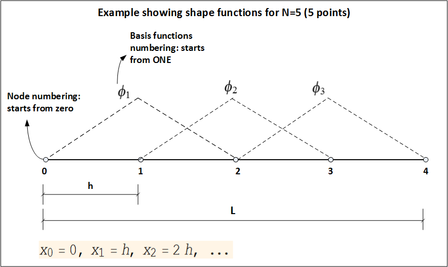
For \(x=\left [ 0,L\right ] \) where \(L\) is the length, we define the shape functions (called tent function in this case) as shown
below
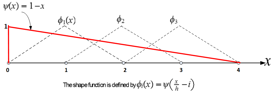
The shape function is defined by \(\phi _{i}\left ( x\right ) =\psi \left ( \frac {x}{h}-i\right ) \) where
\begin{equation} \psi \left ( z\right ) =\left \{ \begin {array} [c]{cc}1-z & \ \ \ \ 0<z<1\\ 0 & z>1 \end {array} \right . \tag {1}\end{equation}
And \(\psi \left ( z\right ) =\psi \left ( -z\right ) \) as shown in this diagram
Now the derivative of \(\phi _{i}^{\prime }\left ( x\right ) \) is given by
\[ \phi _{i}^{\prime }\left ( x\right ) =\left \{ \begin {array} [c]{cc}\frac {1}{h} & (i-1)h<x\leq i\ h\\ -\frac {1}{h} & i\ h<x<\left ( i+1\right ) h\\ 0 & otherwise \end {array} \right . \]
Now we write the weak form in terms of the above shape function (which is our admissible
direction). From part 1 we had
\[ I=\int _{0}^{L}y^{\prime }\left ( x\right ) \phi ^{\prime }\left ( x\right ) +q\ y\left ( x\right ) \phi \left ( x\right ) -f\ \phi \left ( x\right ) ~\ dx=0 \]
And Let
\begin{align*} y\left ( x\right ) & ={\displaystyle \sum \limits _{j=1}^{N}} c_{j}\phi _{j}\left ( x\right ) \\ y^{\prime }\left ( x\right ) & ={\displaystyle \sum \limits _{j=1}^{N}} c_{j}\phi _{j}^{\prime }\left ( x\right ) \end{align*}
Hence, now we pick one admissible direction at a time, and need to satisfy the above integral for
each of these. Hence we write
\[ I_{j}=\int _{0}^{L}\left ( {\displaystyle \sum \limits _{i=1}^{N}} c_{i}\phi _{i}^{\prime }\left ( x\right ) \right ) \phi _{j}^{\prime }\left ( x\right ) +q\ \left ( {\displaystyle \sum \limits _{i=1}^{N}} c_{i}\phi _{i}\left ( x\right ) \right ) \phi _{j}\left ( x\right ) -f\ \phi _{j}\left ( x\right ) ~\ dx=0\ \ \ \ \ \ \ \ j=1,2,\cdots N \]
But due to sphere on influence of the \(\phi _{j}\left ( x\right ) \) extending to only \(x_{j-1}\cdots x_{j+1}\) the above becomes
\[ I_{j}=\int _{x_{j-1}}^{x_{j+1}}\left ( {\displaystyle \sum \limits _{i=j-1}^{j+1}} c_{i}\phi _{i}^{\prime }\left ( x\right ) \right ) \phi _{j}^{\prime }\left ( x\right ) +q\ \left ( {\displaystyle \sum \limits _{i=j-1}^{j+1}} c_{i}\phi _{i}\left ( x\right ) \right ) \phi _{j}\left ( x\right ) -f\ \phi _{j}\left ( x\right ) ~\ dx=0\ \ \ \ \ \ \ \ j=1,2,\cdots N \]
Hence we obtain \(N\) equations which we solve for the \(N\) coefficients \(c_{j}\)
Now to evaluate \(I_{j}\) we write
\begin{align*} I_{j} & =\int _{x_{j-1}}^{x_{j}}\cdots \ dx+\int _{xj}^{x_{j+1}}\cdots \ dx\\ & =\int _{x_{j-1}}^{x_{j}}\left ( {\displaystyle \sum \limits _{i=j-1}^{j}} c_{i}\phi _{i}^{\prime }\left ( x\right ) \right ) \phi _{j}^{\prime }\left ( x\right ) +q\ \left ( {\displaystyle \sum \limits _{i=j-1}^{j}} c_{i}\phi _{i}\left ( x\right ) \right ) \phi _{j}\left ( x\right ) -f\ \phi _{j}\left ( x\right ) ~dx\\ & +\\ & \ \ \int _{x_{j}}^{x_{j}+1}\left ( {\displaystyle \sum \limits _{i=j}^{j+1}} c_{i}\phi _{i}^{\prime }\left ( x\right ) \right ) \phi _{j}^{\prime }\left ( x\right ) +q\ \left ( {\displaystyle \sum \limits _{i=j}^{j+1}} c_{i}\phi _{i}\left ( x\right ) \right ) \phi _{j}\left ( x\right ) -f\ \phi _{j}\left ( x\right ) ~dx \end{align*}
Now we will show the above for \(j=1\) which will be sufficient to build the \(A\) matrix due to
symmetry.
For \(j=1\)
\[ I_{1}=\int _{0}^{2h}\left ( {\displaystyle \sum \limits _{i=1}^{2}} c_{i}\phi _{i}^{\prime }\left ( x\right ) \right ) \phi _{1}^{\prime }\left ( x\right ) +q\ \left ( {\displaystyle \sum \limits _{i=1}^{2}} c_{i}\phi _{i}\left ( x\right ) \right ) \phi _{1}\left ( x\right ) -f\ \phi _{1}\left ( x\right ) ~\ dx\
\]
Hence breaking the interval into 2 parts we obtain
\begin{align*} I_{1} & =\int _{0}^{h}\left ( {\displaystyle \sum \limits _{i=1}^{1}} c_{i}\phi _{i}^{\prime }\left ( x\right ) \right ) \phi _{1}^{\prime }\left ( x\right ) +q\ \left ( {\displaystyle \sum \limits _{i=1}^{1}} c_{i}\phi _{i}\left ( x\right ) \right ) \phi _{1}\left ( x\right ) -f\ \phi _{1}\left ( x\right ) ~\ dx\\ & +\\ & \int _{h}^{2h}\left ( {\displaystyle \sum \limits _{i=1}^{2}} c_{i}\phi _{i}^{\prime }\left ( x\right ) \right ) \phi _{1}^{\prime }\left ( x\right ) +q\ \left ( {\displaystyle \sum \limits _{i=1}^{2}} c_{i}\phi _{i}\left ( x\right ) \right ) \phi _{1}\left ( x\right ) -f\ \phi _{1}\left ( x\right ) \ dx \end{align*}
Hence
\begin{align} I_{1} & =\int _{0}^{h}\left ( c_{1}\phi _{1}^{\prime }\left ( x\right ) \right ) \phi _{1}^{\prime }\left ( x\right ) +q\ \left ( c_{1}\phi _{1}\left ( x\right ) \right ) \phi _{1}\left ( x\right ) -f\ \phi _{1}\left ( x\right ) ~\ dx\nonumber \\ & +\nonumber \\ & \int _{h}^{2h}\left ( c_{1}\phi _{1}^{\prime }\left ( x\right ) +c_{2}\phi _{2}^{\prime }\left ( x\right ) \right ) \phi _{1}^{\prime }\left ( x\right ) +q\ \left ( c_{1}\phi _{1}\left ( x\right ) +c_{2}\phi _{2}\left ( x\right ) \right ) \phi _{1}\left ( x\right ) -f\ \phi _{1}\left ( x\right ) ~\ dx \tag {2}\end{align}
Now set up a little table to do the above integral.
| | | | |
| Range |
\(\phi _{1}^{\prime }\) |
\(\phi _{2}^{\prime }\) |
\(\phi _{1}\) |
\(\phi _{2}\) |
| | | | |
| \(\left [ 0,h\right ] \) | \(\frac {1}{h}\) | \(N/A\) | \(\psi \left ( -\frac {x}{h}+1\right ) \rightarrow \frac {x}{h}\) | \(N/A\) |
| | | | |
| \(\left [ h,2h\right ] \) | \(\frac {-1}{h}\) | \(\frac {1}{h}\) | \(\psi \left ( \frac {x}{h}-1\right ) \rightarrow 2-\frac {x}{h}\) | \(\psi \left ( -\frac {x}{h}+2\right ) \rightarrow \frac {x}{h}-1\) |
| | | | |
The above table was build by noting that for \(\phi _{j},\) it will have the equation \(\psi \left ( \frac {x}{h}-i\right ) \) when \(x\) is under the left leg
of tent. And it will have the equation \(\psi \left ( -\frac {x}{h}+i\right ) \) when \(x\) is under the right leg of the tent. This is because for \(x<0\),
the argument to \(\psi ()\) is negative and so we flip the argument as per the definition for \(\psi \) shown in the
top of this report.
Hence we obtain for the integral in (2)
\begin{align*} I_{1} & =\int _{0}^{h}\left [ c_{1}\left ( \frac {1}{h}\right ) \right ] \left ( \frac {1}{h}\right ) +q\ \left ( c_{1}\frac {x}{h}\right ) \frac {x}{h}-f\ \frac {x}{h}~\ dx\\ & +\\ & \int _{h}^{2h}\left [ c_{1}\left ( \frac {-1}{h}\right ) +c_{2}\ \left ( \frac {1}{h}\right ) \right ] \ \left ( \frac {-1}{h}\right ) +q\ \left ( c_{1}\left ( 2-\frac {x}{h}\right ) +c_{2}\left ( \frac {x}{h}-1\right ) \right ) \left ( 2-\frac {x}{h}\right ) -f\left ( \ 2-\frac {x}{h}\right ) ~\ dx \end{align*}
so the above becomes integral becomes
\begin{align*} I_{1} & =\int _{0}^{h}\frac {c_{1}}{h^{2}}+q\ c_{1}\left ( \frac {x^{2}}{h^{2}}\right ) -f\frac {x}{h}~\ dx\\ & +\\ & \int _{h}^{2h}\frac {c_{1}}{h^{2}}-\ \frac {c_{2}}{h^{2}}+qc_{1}\left ( 4-4\frac {x}{h}+\frac {x^{2}}{h^{2}}\right ) +qc_{2}\left ( 3\frac {x}{h}-\frac {x^{2}}{h^{2}}-2\right ) -2f\ +f\frac {x}{h}~\ dx \end{align*}
Hence
\begin{align*} I_{1} & =\frac {c_{1}}{h^{2}}\int _{0}^{h}dx+\frac {q}{h^{2}}\ c_{1}\int _{0}^{h}x^{2}dx-\frac {f}{h}\ \int _{0}^{h}xdx\\ & +\\ & \frac {c_{1}}{h^{2}}\int _{h}^{2h}dx-\ \frac {c_{2}}{h^{2}}\int _{h}^{2h}dx+qc_{1}\int _{h}^{2h}\left ( 4-4\frac {x}{h}+\frac {x^{2}}{h^{2}}\right ) dx+qc_{2}\int _{h}^{2h}\left ( 3\frac {x}{h}-\frac {x^{2}}{h^{2}}-2\right ) dx-2f\int _{h}^{2h}dx\ +\frac {f}{h}\int _{h}^{2h}x~\ dx \end{align*}
Which becomes
\begin{align*} I_{1} & =\frac {c_{1}}{h^{2}}h+\frac {q}{h^{2}}\ c_{1}\left ( \frac {1}{3}h^{3}\right ) -\frac {f}{2h}h^{2}~\\ & +\\ & \frac {c_{1}}{h^{2}}h-\ \frac {c_{2}}{h^{2}}h+qc_{1}\left ( 4h-2\frac {3h^{2}}{h}+\frac {1}{3}\frac {7h^{3}}{h^{2}}\right ) +qc_{2}\left ( \frac {3}{2h}\left ( 3h^{2}\right ) -\frac {1}{3h^{2}}\left ( 7h^{3}\right ) -2h\right ) -2fh\ +\frac {f}{2h}3h^{2}\end{align*}
or
\begin{align*} I_{1} & =\frac {c_{1}}{h}+c_{1}\ \frac {qh}{3}-\frac {f}{2}h~\\ & +\\ & \frac {c_{1}}{h}-\ \frac {c_{2}}{h}+qc_{1}\left ( 4h-6h+\frac {7}{3}h\right ) +qc_{2}\left ( \frac {9h}{2}-\frac {7}{3}h-2h\right ) -2fh\ +\frac {3f}{2}h~\
\end{align*}
Therefore
\[ I_{1}=\frac {c_{1}}{h}+c_{1}\ \frac {qh}{3}+\frac {c_{1}}{h}-\ \frac {c_{2}}{h}+qc_{1}\left ( \frac {1}{3}h\right ) +qc_{2}\left ( \frac {1}{6}h\right ) -fh~ \]
Hence
\[ I_{1}=c_{1}\left ( \frac {2}{h}+\frac {2}{3}qh\right ) +c_{2}\left ( -\frac {1}{h}+\frac {1}{6}qh\right ) -fh=0 \]
Multiply by \(h\) we obtain
\begin{equation} \fbox {$I_{1}=c_{1}\left ( 2+\frac {2}{3}h^{2}q\right ) +c_{2}\left ( -1+\frac {1}{6}h^{2}q\right ) -fh^{2}=0$} \tag {2}\end{equation}
Hence we now can set up the \(Ax=b\) system using only the above equation by taking advantage that \(A\) will
be tridiagonal and there is symmetry along the diagonal.
\[\begin {bmatrix} \left ( 2+\frac {2}{3}h^{2}q\right ) & \left ( -1+\frac {1}{6}h^{2}q\right ) & 0 & 0 & \cdots & 0\\ \left ( -1+\frac {1}{6}h^{2}q\right ) & \left ( 2+\frac {2}{3}h^{2}q\right ) & \left ( -1+\frac {1}{6}h^{2}q\right ) & 0 & \cdots & 0\\ 0 & \left ( -1+\frac {1}{6}h^{2}q\right ) & \left ( 2+\frac {2}{3}h^{2}q\right ) & \left ( -1+\frac {1}{6}h^{2}q\right ) & \cdots & 0\\ 0 & 0 & 0 & 0 & \ddots & \vdots \\ 0 & 0 & 0 & \cdots & \left ( -1+\frac {1}{6}h^{2}q\right ) & \left ( 2+\frac {2}{3}h^{2}q\right ) \end {bmatrix}\begin {bmatrix} c_{1}\\ c_{2}\\ c_{3}\\ \vdots \\ c_{N}\end {bmatrix} =fh^{2}\begin {bmatrix} 1\\ 1\\ 1\\ \vdots \\ 1 \end {bmatrix} \]
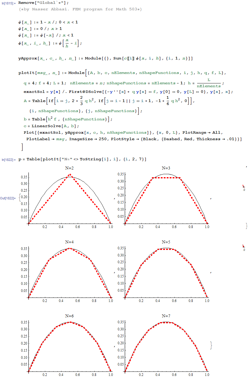
The following is the FEM program to implement the above, with few plots showing how close it
gets to the real solution as \(N\) increases.
I also written a small Manipulate program to simulate the above. Here it is